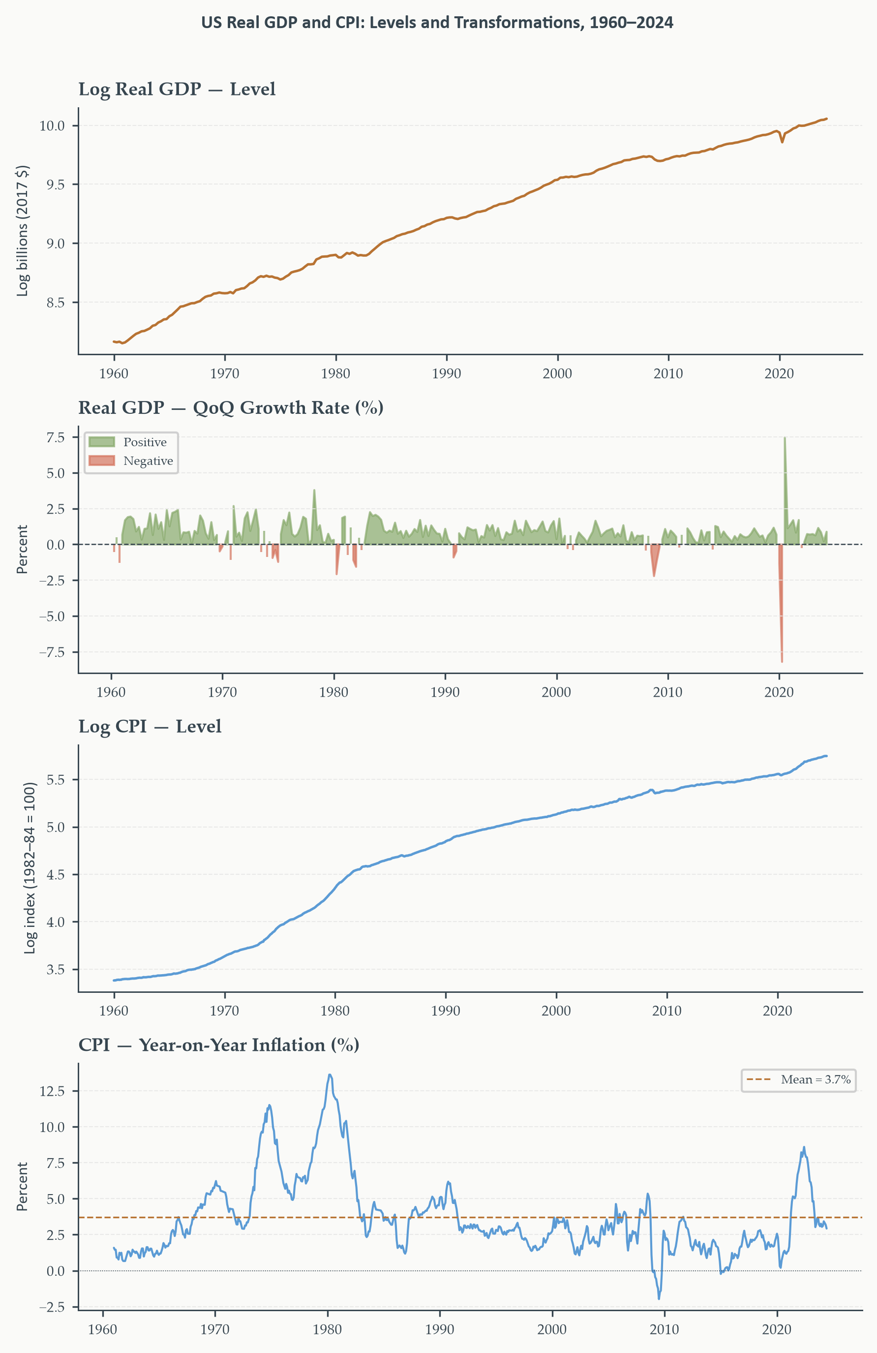
---
title: "Foundations of Time Series Analysis"
author: ""
abstract: |
Time series analysis is the discipline of extracting information from the past to say something credible about the future. This chapter establishes the conceptual and mathematical foundations on which the entire course rests: what time series data are and how they differ from other data structures, what forecasting is and is not, and how the mathematical machinery of difference equations governs the behavior of time series processes. A central result — connecting difference equations to linear algebra — is that the stability of any linear time series model is determined by the eigenvalues of its companion matrix, a fact that links directly to the economic concepts of stationarity and unit roots that underpin modern macroeconometrics.
jupyter: python3
format:
html:
toc: true
toc-depth: 3
toc-title: "In this chapter"
number-sections: true
code-fold: true
code-summary: "Show code"
code-tools: true
theme: cosmo
css: styles.css
highlight-style: github
fig-align: center
fig-cap-location: bottom
fig-responsive: true
html-math-method: mathjax
embed-resources: false
execute:
echo: true
warning: false
message: false
cache: false
---
```{python}
#| label: setup
#| include: false
import numpy as np
import pandas as pd
import matplotlib.pyplot as plt
import matplotlib as mpl
import matplotlib.ticker as mticker
from statsmodels.tsa.stattools import adfuller, kpss
from statsmodels.graphics.tsaplots import plot_acf, plot_pacf
import pandas_datareader.data as web
from datetime import datetime
import warnings
warnings.filterwarnings("ignore")
# ── EO Brand Palette ───────────────────────────────────────────────────────────
EO_CHARCOAL = "#36454F"
EO_COPPER = "#B87333"
EO_SAGE = "#87A96B"
EO_SKYBLUE = "#5B9BD5"
EO_TERRACOTTA = "#D4745E"
EO_LAVENDER = "#8E7AB5"
EO_COLORS = [EO_COPPER, EO_SKYBLUE, EO_SAGE,
EO_TERRACOTTA, EO_LAVENDER, EO_CHARCOAL]
# Page background matching CSS light-mode (#FAFAF8)
PAGE_BG = "#FAFAF8"
# ── Global rcParams ────────────────────────────────────────────────────────────
mpl.rcParams.update({
"figure.figsize": (6, 3),
"figure.dpi": 150,
"figure.facecolor": PAGE_BG,
"figure.edgecolor": PAGE_BG,
"axes.facecolor": PAGE_BG,
"axes.edgecolor": EO_CHARCOAL,
"axes.linewidth": 0.7,
"axes.grid": True,
"axes.grid.axis": "y",
"axes.spines.top": False,
"axes.spines.right": False,
"axes.titlesize": 9,
"axes.titleweight": "bold",
"axes.titlecolor": EO_CHARCOAL,
"axes.titlelocation": "left",
"axes.labelsize": 8,
"axes.labelcolor": EO_CHARCOAL,
"axes.labelweight": "normal",
"axes.prop_cycle": mpl.cycler(color=EO_COLORS),
"grid.color": "#E5E5E5",
"grid.linewidth": 0.5,
"grid.linestyle": "--",
"grid.alpha": 0.8,
"xtick.color": EO_CHARCOAL,
"ytick.color": EO_CHARCOAL,
"xtick.labelsize": 7,
"ytick.labelsize": 7,
"xtick.direction": "out",
"ytick.direction": "out",
"xtick.major.size": 3,
"ytick.major.size": 3,
"lines.linewidth": 1.2,
"lines.solid_capstyle": "round",
"legend.frameon": True,
"legend.framealpha": 0.9,
"legend.edgecolor": "#CCCCCC",
"legend.facecolor": PAGE_BG,
"legend.fontsize": 6,
"legend.title_fontsize": 6,
"font.family": "serif",
"font.serif": ["Palatino Linotype", "Palatino", "Georgia",
"DejaVu Serif"],
"font.sans-serif": ["Calibri", "Arial", "DejaVu Sans"],
"font.size": 8,
"text.color": EO_CHARCOAL,
"savefig.dpi": 300,
"savefig.bbox": "tight",
"savefig.facecolor": PAGE_BG,
})
def eo_suptitle(fig, title, **kwargs):
defaults = dict(fontsize=9, fontweight="bold",
color=EO_CHARCOAL, fontfamily="Calibri", y=1.01)
defaults.update(kwargs)
fig.suptitle(title, **defaults)
def eo_style_ax(ax):
for obj in [ax.title, ax.xaxis.label, ax.yaxis.label]:
obj.set_fontfamily("Calibri")
```
```{python}
#| label: data-download
#| include: false
#| cache: true
from pathlib import Path
DATA_PATH = Path("../../data/raw")
start = datetime(1960, 1, 1)
end = datetime(2024, 6, 30)
gdp = pd.read_csv(DATA_PATH / "GDPC1.csv", index_col="date", parse_dates=True).loc[str(start):str(end)]
cpi = pd.read_csv(DATA_PATH / "CPIAUCSL.csv", index_col="date", parse_dates=True).loc[str(start):str(end)]
gdp.columns = ["Real GDP"]
cpi.columns = ["CPI"]
gdp["Log Real GDP"] = np.log(gdp["Real GDP"])
gdp["GDP Growth (QoQ)"] = gdp["Log Real GDP"].diff() * 100
cpi["Log CPI"] = np.log(cpi["CPI"])
cpi["Inflation (YoY)"] = cpi["Log CPI"].diff(12) * 100
```
::: {.callout-note}
## Learning Objectives
By the end of this chapter, you will be able to:
- Distinguish time series data from cross-sectional and panel data, and explain why temporal ordering changes the nature of statistical inference
- Define forecasting precisely, differentiate it from prediction and causal inference, and identify the three types of forecasts: point, interval, and density
- Explain the role of the loss function in determining the optimal forecast, and show why squared error loss and absolute error loss lead to different optimal forecasts
- Articulate the particular challenges that make economic forecasting hard, including structural change, measurement error, the Lucas critique, and deep parameters
- Use standard time series notation, including the lag and difference operators, fluently and correctly
- Define white noise, distinguish IID noise from weak white noise, and explain why the difference matters in practice
- Solve first-order and higher-order linear difference equations using the companion matrix representation, identify their eigenvalues, and classify the dynamic behavior as stable, unit-root, or explosive
- Define strict and weak stationarity, explain why stationarity matters for estimation and inference, and identify the main types of nonstationarity in economic data
- Compute, plot, and interpret the sample ACF and PACF for an observed time series
- Apply the ADF and KPSS tests to assess whether a series is stationary, and interpret their results jointly
- Apply the appropriate transformation to achieve stationarity and explain its economic interpretation
:::
## What Is a Time Series?
### Data with a Memory
Here is a question that seems almost too simple to be worth asking: what makes [time series](https://en.wikipedia.org/wiki/Time_series) data different from any other kind of data?
The answer is not the subject matter. It is not that time series involve economics, or finance, or any particular domain. The answer is that time series data have a memory. Each observation is connected to the ones that came before it, and that connection is not a statistical nuisance to be corrected — it is the signal we are trying to model. Strip away the temporal ordering, and you have destroyed the most important thing the data contain.
This is what separates time series analysis from the rest of [econometrics](https://en.wikipedia.org/wiki/Econometrics). In a standard regression course, the ideal dataset is one where every observation is an independent draw from some population — where knowing one row of the spreadsheet tells you nothing about any other row. In time series analysis, the exact opposite is true. We want the rows to be connected. We are trying to measure, model, and exploit those connections to say something useful about observations we have not yet seen.
That shift in orientation — from independence as an assumption to dependence as the object of study — has consequences for every tool in the econometrician's toolkit. Estimators change. Standard errors change. Tests change. Even the questions we ask change. Understanding why requires starting from first principles, and first principles require getting clear on what kind of data we are actually working with.
### Types of Datasets: Cross-Sectional, Time Series, and Panel Data
Economists work with three fundamental types of data, and keeping them distinct is essential for choosing the right methods.
**[Cross-sectional data](https://en.wikipedia.org/wiki/Cross-sectional_data)** capture many units at a single point in time. A survey of household incomes in 2023, a snapshot of firms' balance sheets at the end of a fiscal year, the GDP of 150 countries in a given quarter — these are all cross-sectional. The organizing dimension is breadth: many observations of different units, all contemporaneous. The core statistical challenge is ensuring that units are representative of some population of interest, and that apparent relationships are not confounded by omitted factors. The standard assumption — sometimes heroic, but analytically necessary — is that observations are independent of each other.
**Time series data** follow a single unit — or a small number of units — across many points in time. US real GDP from 1947 to the present, the daily closing price of an equity index over ten years, the monthly unemployment rate for Germany since reunification — these are time series. The organizing dimension is depth: many observations of the same unit, ordered sequentially through time. The core statistical challenge is dependence: today's observation is connected to yesterday's, which was connected to the day before that. This dependence is not a flaw in the data; it is the feature we are trying to understand.
::: {.callout-note}
## Definition 1.1 — Time Series
A **time series** is a collection of observations $\{y_t\}_{t=1}^{T}$, where $y_t$ denotes the value of the variable of interest at time index $t$, and the index $t$ runs from $1$ to $T$ in a fixed, ordered sequence. The subscript $t$ is not a label — it encodes the temporal position of each observation and cannot be permuted without destroying the data's structure.
:::
**[Panel data](https://en.wikipedia.org/wiki/Panel_data)** (sometimes called longitudinal data) combine both dimensions: many units, each observed across many time periods. Following 50 US states over 30 years, tracking a sample of 10,000 workers over their careers, observing the quarterly earnings of 500 publicly traded firms across two decades — these are panel datasets. Their power lies in the combination: the time dimension allows researchers to control for unobserved unit-specific characteristics (fixed effects) that would confound a pure cross-sectional analysis, while the cross-sectional dimension provides variation that a pure time series cannot.
::: {.callout-note}
## Definition 1.2 — Panel Data
A **panel dataset** is a collection of observations $\{y_{it}\}$ where $i = 1, \ldots, N$ indexes units and $t = 1, \ldots, T$ indexes time periods. A **balanced panel** has $N \times T$ observations. An **unbalanced panel** has gaps: some units are missing in some periods.
:::
The critical difference for our purposes: in a panel, cross-sectional variation helps identify parameters that would be hard to pin down from a single series. In time series analysis, we must extract all information from the temporal variation of one — or a few — series. This constraint is not a weakness; it is a discipline that forces precision about the structure of the data-generating process. This course focuses on time series analysis; panel methods belong to a separate econometrics course.
### A Gallery of Economic and Financial Time Series
Before formalizing any of these ideas, it is worth spending a moment with the kinds of data this course is actually about. Each series below illustrates a different feature that will become analytically important as the course develops.
**Real Gross Domestic Product (quarterly).** GDP measures the total value of goods and services produced in an economy over a quarter. US real GDP has grown persistently over the postwar period, punctuated by recessions — in 1980–82, 1990–91, 2001, 2008–09, and most dramatically in early 2020. The level has no fixed mean and no fixed variance; it trends upward through time. We will typically work with the growth rate — the percentage change from one quarter to the next — which fluctuates around a stable, if modest, positive mean.
**Consumer Price Index (monthly).** The CPI tracks the cost of a fixed basket of goods and services. Like GDP, its level grows almost continuously and has no stable mean. But the rate of change — inflation — behaves very differently across periods. The 1970s saw high, volatile inflation. The 1990s and 2000s brought a long era of low, stable inflation. The years 2021–2023 brought the sharpest inflation since the 1970s. Whether the inflation rate itself is stationary is one of the most actively debated empirical questions in macroeconometrics, and we return to it later in this chapter.
**Equity index returns (daily).** The daily percentage return on a broad stock market index fluctuates around a near-zero mean with no obvious trend. But large movements tend to be followed by more large movements — in either direction — a phenomenon known as **volatility clustering**. This dependence in the second moment, but not the first, is the hallmark of ARCH and GARCH models studied later in the course.
**Nominal exchange rates (daily).** The nominal exchange rate between two major currencies evolves as something close to a random walk: today's rate is the best predictor of tomorrow's, and changes are small and largely unpredictable. Exchange rates are a canonical example of a unit root process, and their near-unpredictability is closely connected to the efficient markets hypothesis.
**Term structure of interest rates (monthly).** Interest rates at different maturities move together but not in lockstep. The spread between long-term and short-term rates — the yield curve — has one of the strongest track records as a leading indicator of US recessions: when it inverts, recession tends to follow within twelve to eighteen months.
What these series share is that they are all ordered by time, all exhibit some form of temporal dependence, and all require tools designed specifically for that dependence. What distinguishes them — trends, cycles, volatility clustering, unit roots, seasonal patterns — is exactly what this course will teach us to characterize and model.
## What Is Forecasting?
[Forecasting](https://en.wikipedia.org/wiki/Forecasting) means using what we know today to say something credible about tomorrow. It sounds simple, and in some settings it is. A meteorologist uses today's atmospheric conditions to forecast tomorrow's weather. A shipping company uses historical demand patterns to forecast container volumes next month. In economics and finance the same logic applies — but the execution is considerably harder, for reasons we examine shortly. Before getting there, it is worth being precise about what forecasting actually is, and distinguishing it carefully from two activities it is frequently confused with: cross-sectional prediction and causal inference.
### Forecasting vs. Prediction
In the machine learning literature, "[prediction](https://en.wikipedia.org/wiki/Prediction#)" refers to a cross-sectional exercise: using a set of observable features — income, age, education, location — to predict an outcome for a new individual. The time dimension is absent. The challenge is finding the right features and the right model, and performance is measured by how well the model generalizes to new units from the same population.
Forecasting is a fundamentally different exercise. We observe a sequence $y_1, y_2, \ldots, y_T$ and want to say something about $y_{T+1}, y_{T+2}, \ldots$ — values of the same variable, for the same unit, at future points in time. The conditioning set is a history, not a cross-section of features. The challenge is temporal extrapolation: using what the past behavior of a series tells us about its future behavior.
A model that fits historical data brilliantly may still fail as a forecast if it has captured features of the sample period that do not persist. This is the time-series version of overfitting, and it is one of the most persistent hazards in applied forecasting work.
### Forecasting vs. Causal Inference
[Causal inference](https://en.wikipedia.org/wiki/Causal_inference) asks: if we intervene and change $X$, what happens to $Y$? Answering this requires credible identification of a causal mechanism — a randomized experiment, a natural experiment, an instrumental variable — that separates the effect of $X$ from confounders.
Forecasting asks only: given everything we observe up to time $T$, what is our best guess of $Y$ at time $T + h$? This is an exercise in conditional expectation, not causal identification. A variable can be a powerful predictor without causing $Y$. And a genuine cause can be a poor predictor if it operates with long and uncertain lags, or if it is itself difficult to forecast.
::: {.callout-warning icon=false}
## A Common Mistake
A finding that lagged values of $X$ help forecast $Y$ is tempting to interpret as evidence that $X$ causes $Y$. It is not. It says only that $X$ contains information about the future path of $Y$. Granger causality, which we study later in the course, formalizes this predictive notion precisely, and deliberately avoids claiming anything about true causation.
:::
### Types of Forecasts
**Point forecasts.** A point forecast is a single number: our best guess of $y_{T+h}$ given everything we know at time $T$. If $\mathcal{F}_T$ denotes the information set available at time $T$, the optimal point forecast under **squared error loss** is the conditional expectation:
$$\hat{y}_{T+h|T} = \mathbb{E}[y_{T+h} \mid \mathcal{F}_T]$$
The quantity $h$ is the **forecast horizon**. A one-step-ahead forecast has $h = 1$; a four-quarter-ahead forecast for quarterly data has $h = 4$. Point forecasts are the most common form in practice, but also the most incomplete — they say nothing about how confident we should be.
**Interval forecasts.** An interval forecast reports a range $[L_{T+h},\, U_{T+h}]$ within which the true value $y_{T+h}$ is expected to fall with some specified probability — typically 80% or 95%. These **prediction intervals** describe uncertainty about a future realization, not about an estimated parameter. For a Gaussian process, a $(1-\alpha)$ prediction interval takes the form:
$$\hat{y}_{T+h|T} \;\pm\; z_{\alpha/2} \cdot \hat{\sigma}_{T+h|T}$$
**Density forecasts.** The most complete type of forecast is a full probability distribution over future values: $\hat{p}(y_{T+h} \mid \mathcal{F}_T)$. A density forecast encodes the entire shape of our uncertainty — including skewness and the probability of extreme outcomes. It is particularly valuable in risk management and monetary policy, where the tails of the distribution matter as much as the center.
### The Particular Challenges of Economic Forecasting
Economic forecasting is genuinely hard — harder than weather forecasting, harder than most engineering applications. Understanding why is essential for calibrating what we should expect from our models.
**Structural change.** The relationships between economic variables are not fixed laws of nature. They evolve as institutions change, technology changes, and the policy environment changes. A model estimated over one historical period may perform poorly in a later period not because it was misspecified for the earlier period, but because the economy itself changed.
**Measurement error and data revisions.** Economic data are rarely final when first released. GDP figures are revised — sometimes substantially — months and years after initial publication. A model that fits the revised, final data well may have performed quite differently in real time, when only the preliminary release was available.
**The [Lucas critique](https://en.wikipedia.org/wiki/Lucas_critique) and deep parameters.** In a [1976 paper](https://people.sabanciuniv.edu/atilgan/FE500_Fall2013/2Nov2013_CevdetAkcay/LucasCritique_1976.pdf) that changed the course of macroeconomics, [Robert Lucas](https://en.wikipedia.org/wiki/Robert_Lucas_Jr.) argued that the behavioral relationships estimated from historical data — how consumers respond to income changes, how firms respond to interest rates — are not structural. They are reduced-form coefficients that reflect agents' optimization under a particular policy regime. When the regime changes, agents reoptimize, and the historical relationships break down.
The key concept underlying Lucas's argument is the distinction between **deep parameters** and estimated behavioral coefficients. Deep parameters — preferences, technology, information sets — are genuinely structural: they are invariant to changes in the policy environment because they describe the primitive characteristics of households and firms. Estimated behavioral equations, by contrast, are composites of deep parameters and the specific constraints agents face under a given regime. Change the regime, and the estimated coefficients change too, even if the deep parameters do not.
This is why modern macroeconomics has moved toward structural models that explicitly identify deep parameters, and why even purely statistical forecasting models should be interpreted with the Lucas critique in mind: they are approximations that work well within a stable regime and may fail when the regime shifts.
**Reflexivity.** In the natural sciences, the process being observed does not read the forecast. In economics, it does. A central bank that publishes an inflation forecast influences inflation expectations, which influence wage negotiations and price-setting, which influence actual inflation. This feedback from forecasts to outcomes has no clean analogue in the physical sciences.
None of these challenges makes economic forecasting worthless. The question is never whether a forecast is perfect — no forecast is — but whether it is better than the available alternatives, and by how much.
### The Loss Function: A Conceptual Introduction
We said that the optimal point forecast under squared error loss is the conditional mean $\mathbb{E}[y_{T+h} \mid \mathcal{F}_T]$. But why squared error loss? And does the choice of loss function actually matter?
The answer is yes — it matters substantially. The **[loss function](https://en.wikipedia.org/wiki/Loss_function)** $\mathcal{L}(e_{T+h})$, where $e_{T+h} = y_{T+h} - \hat{y}_{T+h|T}$ is the forecast error, encodes our preferences over different kinds of mistakes. Different preferences lead to different optimal forecasts.
Under **squared error loss**, $\mathcal{L}(e) = e^2$: errors are penalized symmetrically, and large errors are penalized disproportionately. Under **absolute error loss**, $\mathcal{L}(e) = |e|$: the penalty is linear in the error size. Under **asymmetric loss**, over- and under-forecasting are penalized differently — a central bank that finds unexpected inflation more costly than unexpected deflation, or a supply-chain manager for whom stockouts cost far more than excess inventory, faces this structure.
::: {.callout-note}
#### Why Squared Loss Gives the Mean and Absolute Loss Gives the Median
**Squared error loss.** We want to find the constant $m$ minimizing $\mathbb{E}[(y - m)^2]$. Expanding and differentiating with respect to $m$:
$$\frac{d}{dm}\,\mathbb{E}[(y-m)^2] = -2\mathbb{E}[y] + 2m = 0 \implies m = \mathbb{E}[y]$$
The **conditional mean** minimizes expected squared error.
**Absolute error loss.** We want to minimize $\mathbb{E}[|y - m|] = \int_{-\infty}^{m}(m-y)f(y)\,dy + \int_{m}^{\infty}(y-m)f(y)\,dy$. Differentiating under the integral:
$$\frac{d}{dm}\,\mathbb{E}[|y-m|] = F(m) - [1 - F(m)] = 0 \implies F(m) = \tfrac{1}{2}$$
The value of $m$ where the CDF equals $1/2$ is by definition the **median**. The conditional median minimizes expected absolute error.
The intuition: squared loss penalizes large errors quadratically, pulling the optimal forecast toward the mean to avoid catastrophic misses. Absolute loss penalizes all errors proportionally, making the optimal forecast robust to extremes — the median is not affected by how far outliers sit from the center.
:::
Specifying the loss function is not a technical afterthought — it is a modeling choice determined by the decision problem at hand. We return to loss functions in the chapter on forecast evaluation.
## Notation, Operators, and Key Concepts
### The Time Index and Notation
Every time series analysis begins with a convention for labeling observations in time. The **time index** $t$ runs over some ordered discrete set — $\mathcal{T} = \{1, 2, \ldots, T\}$ for a finite sample, or $\mathcal{T} = \mathbb{Z}$ for the theoretical process underlying the data.
The time index is not just a label. Arithmetic on the index is meaningful: $y_t - y_{t-1}$ is the change from one period to the next; $y_{t-12}$ is the value exactly one year ago (for monthly data); $y_{T+h}$ is the value $h$ periods beyond the end of the sample. The **information set** $\mathcal{F}_t$ denotes everything observable at time $t$ — the current value $y_t$, all past values $y_{t-1}, y_{t-2}, \ldots$, and possibly other relevant variables.
We will use the following notation consistently throughout the course:
- $\mu = \mathbb{E}[y_t]$: the mean of the process
- $\gamma(h) = \text{Cov}(y_t, y_{t-h})$: the autocovariance at lag $h$
- $\rho(h) = \text{Corr}(y_t, y_{t-h})$: the autocorrelation at lag $h$
- $\sigma^2 = \text{Var}(y_t)$: the variance of the process
- $\varepsilon_t$: an error or innovation term
### Frequency and Regularity
The **frequency** of a time series is how often observations are recorded:
| Frequency | Observations per year | Typical use |
|-----------|-----------------------|-----------------------------------------------|
| Annual | 1 | Long-run growth, cross-country comparisons |
| Quarterly | 4 | GDP, national accounts, monetary policy |
| Monthly | 12 | CPI, unemployment, industrial production |
| Weekly | ~52 | Initial jobless claims, financial flows |
| Daily | ~252 (trading days) | Asset prices, exchange rates |
| Intraday | Thousands | High-frequency trading, market microstructure |
: Common time series frequencies in economics and finance {#tbl-frequencies}
A time series is **regular** if observations are equally spaced in time. Most macroeconomic data are regular. Some financial series are **irregular** — individual transaction records arrive whenever a trade is executed — requiring specialized methods we will not cover in this course.
### The Lag Operator
The most important notational device in time series analysis is the **[lag operator](https://en.wikipedia.org/wiki/Lag_operator)** $L$, defined by:
$$Ly_t = y_{t-1}$$
Applying it $k$ times gives $L^k y_t = y_{t-k}$. We also define $L^{-1}y_t = y_{t+1}$ — the forward shift. A polynomial in $L$,
$$\phi(L) = \phi_0 + \phi_1 L + \phi_2 L^2 + \cdots + \phi_p L^p$$
maps a time series to a linear combination of its current and past values:
$$\phi(L)y_t = \phi_0 y_t + \phi_1 y_{t-1} + \phi_2 y_{t-2} + \cdots + \phi_p y_{t-p}$$
This compact notation becomes indispensable when writing time series models in Chapter 3.
### The Difference Operator
The **first [difference operator](https://en.wikipedia.org/wiki/Recurrence_relation#difference_operator)** $\Delta$ is:
$$\Delta y_t = y_t - y_{t-1} = (1 - L)y_t$$
The equality $\Delta = 1 - L$ holds in the algebra of lag operators. Differencing removes a linear trend. The **second difference** $\Delta^2 y_t = (1-L)^2 y_t = y_t - 2y_{t-1} + y_{t-2}$ removes a quadratic trend. In practice, one round of differencing is almost always sufficient for economic time series.
The **seasonal difference operator** removes seasonal patterns. For monthly data:
$$\Delta_{12} y_t = y_t - y_{t-12} = (1 - L^{12})y_t$$
compares each month to the same month a year earlier. For quarterly data, $\Delta_4 y_t = y_t - y_{t-4}$ does the same.
## White Noise {#sec-whitenoise}
Before developing the mathematics of difference equations, we need a formal baseline: the simplest stationary process, one with no temporal dependence whatsoever. This is [white noise](https://en.wikipedia.org/wiki/White_noise) — the absence of pattern in time, and the building block from which every time series model in this course is constructed.
::: {.callout-note}
## Definition 1.3 — White Noise
A process $\{\varepsilon_t\}$ is a **white noise process** with mean zero and variance $\sigma^2$ if:
1. $\mathbb{E}[\varepsilon_t] = 0$ for all $t$
2. $\text{Var}(\varepsilon_t) = \sigma^2 < \infty$ for all $t$
3. $\text{Cov}(\varepsilon_t, \varepsilon_s) = 0$ for all $t \neq s$
We write $\varepsilon_t \sim WN(0, \sigma^2)$. Its autocovariance function is $\gamma(h) = \sigma^2$ for $h=0$ and $\gamma(h) = 0$ for $h \neq 0$.
:::
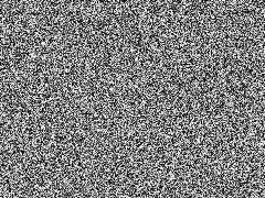
The three conditions are purely about moments — mean, variance, and cross-period covariances. No pattern, no memory, no structure. The image below illustrates what this looks like in a familiar domain: each pixel's intensity is an independent random draw, uncorrelated with every neighboring pixel in every direction. There is nothing to see — no edges, no gradients, no clusters — because by construction there is nothing there. This is the spatial analogue of zero autocorrelation: knowing the intensity of one pixel tells you nothing about any other.
{#fig-spatial-wn width="55%"}
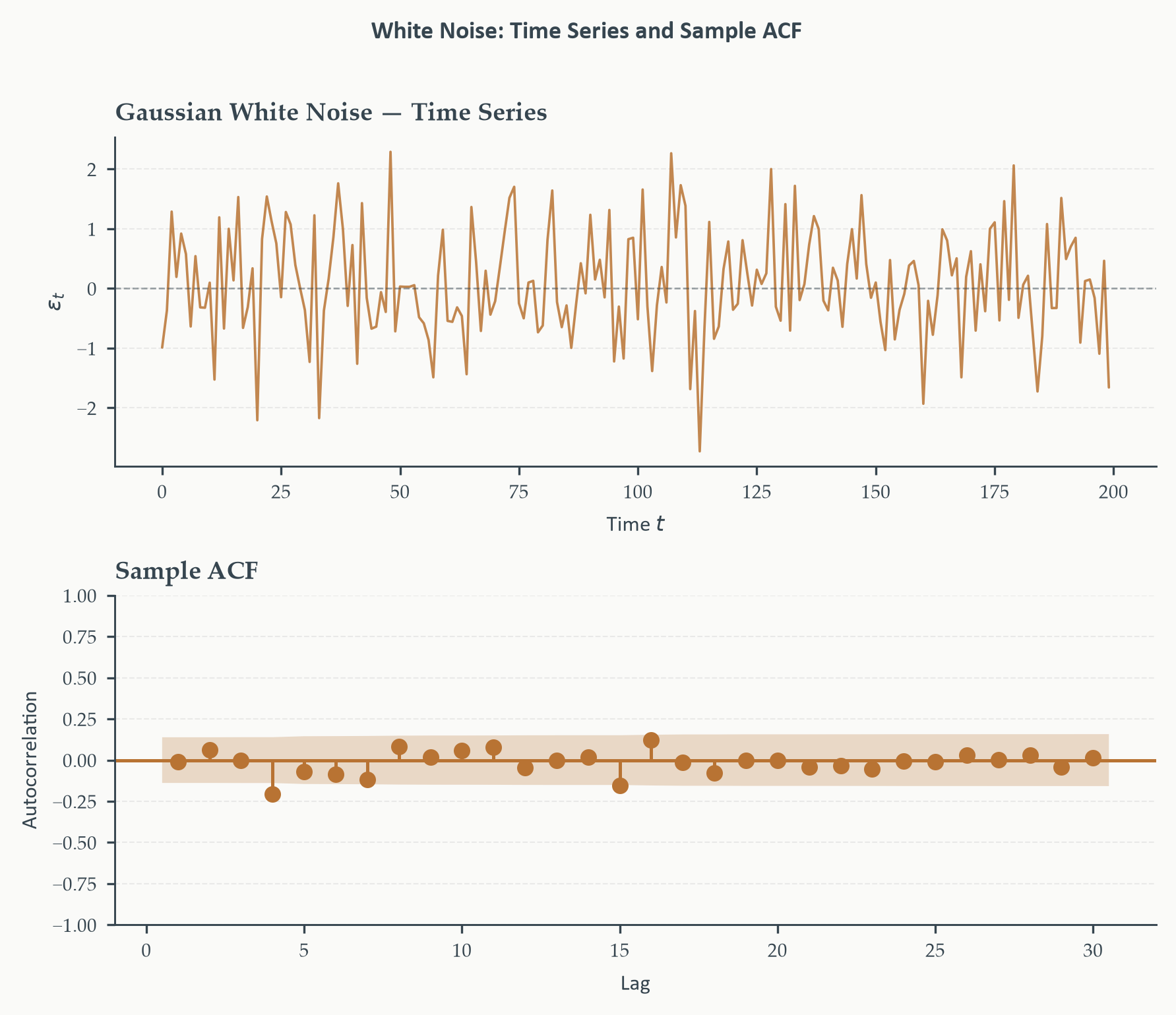
What does white noise look like as a time series? The figure below simulates a simple Gaussian white noise sequence — $\varepsilon_t \overset{\text{iid}}{\sim} N(0,1)$ — and plots it alongside its sample ACF. Two features are immediately visible. First, the time series fluctuates erratically around zero with no discernible trend, cycle, or pattern. Second, the ACF shows no significant spikes at any lag — every bar lies within the 95% confidence bands, confirming that no linear relationship exists between any two observations. This is the time-series counterpart of the spatial image above: pure noise, no memory.
```{python}
#| label: fig-wn-series
#| fig-cap: "A simulated Gaussian white noise series ($T=200$) and its sample ACF. The time plot shows erratic fluctuations around zero with no discernible structure. The ACF confirms this: all autocorrelations lie within the 95% confidence bands (terracotta dashed lines), indicating no statistically significant linear dependence at any lag. This is what a well-specified model's residuals should look like."
#| fig-width: 6
#| fig-height: 5
#| code-fold: true
#| code-summary: "Show code — White noise time series"
from statsmodels.graphics.tsaplots import plot_acf

rng = np.random.default_rng(seed=123)
T   = 200
wn  = rng.normal(0, 1, T)

fig, axes = plt.subplots(2, 1, figsize=(6, 5))

# Time plot
ax = axes[0]
ax.plot(np.arange(T), wn, color=EO_COPPER, linewidth=0.9, alpha=0.85)
ax.axhline(0, color=EO_CHARCOAL, linewidth=0.6, linestyle="--", alpha=0.5)
ax.set_title("Gaussian White Noise — Time Series")
ax.set_xlabel("Time $t$")
ax.set_ylabel("$\\varepsilon_t$")
eo_style_ax(ax)

# ACF
ax = axes[1]
plot_acf(wn, lags=30, ax=ax, color=EO_COPPER,
         vlines_kwargs={"colors": EO_COPPER},
         title="Sample ACF", zero=False, alpha=0.05)
ax.set_xlabel("Lag")
ax.set_ylabel("Autocorrelation")
eo_style_ax(ax)
for line in ax.lines:
    if line.get_linestyle() == "--":
        line.set_color(EO_TERRACOTTA)
        line.set_linewidth(0.8)

eo_suptitle(fig, "White Noise: Time Series and Sample ACF")
fig.tight_layout()
plt.show()
```
**Normality is not required.** It is worth stating explicitly what the definition does not say: white noise places no restriction on the shape of the distribution of $\varepsilon_t$. The three conditions concern only the mean, the variance, and the covariances across time — not the distributional form. A white noise process can be Gaussian, Student-$t$, skewed, heavy-tailed, or have any other shape, as long as it satisfies the three moment conditions. This matters in practice: daily financial returns, for example, are routinely modeled as white noise processes with heavy tails and occasional extreme values — a distribution far from Gaussian — and that is entirely consistent with Definition 1.3. Gaussian white noise is a special and analytically convenient case, not a requirement.
**White noise as a diagnostic tool.** Beyond being a theoretical baseline, white noise plays a central practical role throughout this course: it is the standard we hold our model residuals to. When we fit a time series model — whether an exponential smoother, an ARMA, or a VAR — the residuals $\hat{\varepsilon}_t = y_t - \hat{y}_{t|t-1}$ should behave like white noise if the model has captured all predictable structure in the data. If the residuals are not white noise — if their ACF shows significant autocorrelation at some lags, or if their squared values are correlated — then predictable structure remains in what the model left behind, and a better model exists. In this sense, checking residuals for white noise is not a formality; it is a direct test of whether the model has done its job. The ACF introduced in the next section is the primary tool for performing this check, and we will apply it to model residuals in every subsequent chapter.
**IID noise vs. weak white noise.** White noise as defined above imposes only zero correlation — it says nothing about independence. **IID noise** is stronger: $\varepsilon_t \overset{\text{iid}}{\sim} (0, \sigma^2)$, meaning observations are not just uncorrelated but fully independent and identically distributed. Independence rules out any statistical relationship of any kind, not just linear ones.
The gap matters in practice. It is possible for $\varepsilon_t$ and $\varepsilon_{t-1}$ to be uncorrelated but not independent: knowing $\varepsilon_{t-1}$ tells us nothing about the mean of $\varepsilon_t$, but may tell us something about its variance. This is precisely the situation in ARCH models — residuals are uncorrelated (white noise) but their squared values are correlated. Such residuals pass all standard tests for white noise, which test for zero autocorrelation, while still containing forecastable structure in the second moment. This is why the distinction between IID noise and weak white noise matters for financial time series with volatility clustering.
::: {.callout-tip}
### Hierarchy of White Noise
From strongest to weakest:
$$\text{IID noise} \implies \text{Strong white noise} \implies \text{Weak white noise}$$
For most of this course, we work with weak white noise, noting when stronger assumptions are needed.
:::
## Difference Equations {#sec-diffeq}
### Time Series as Stochastic Difference Equations
This section is the mathematical core of the chapter. The machinery developed here — characteristic roots, companion matrices, eigenvalues, stability conditions — underpins every model in this course. It is worth working through carefully, because the payoff is large: by the end of this section, the concepts of stationarity, unit roots, and explosive processes follow almost as corollaries.
A time series model is, at its core, a **[difference equation (with constant coefficients)](https://en.wikipedia.org/wiki/Linear_recurrence_with_constant_coefficients#Characteristic_equation_and_roots** — a rule relating the current value of a variable to its own past values and possibly to external inputs. A first-order deterministic example:
$$y_t = \phi y_{t-1} + c, \qquad t = 1, 2, 3, \ldots$$
where $\phi$ and $c$ are constants and $y_0$ is a given initial condition. Before doing any algebra, it is worth saying in plain terms what these two parameters are doing. Think of $c$ as the **pull**: the value $y_t$ would converge to if there were no memory at all — a fixed anchor the process is always being drawn toward. Think of $\phi$ as the **push**: the memory factor that keeps $y_t$ close to its own recent past instead of jumping immediately to $c$. A large $|\phi|$ means strong memory and slow convergence toward the anchor; a small $|\phi|$ means weak memory and rapid convergence. The interplay between these two forces — the pull of $c$ and the push of $\phi$ — is what the mathematics below makes precise.
Adding white noise $\varepsilon_t \sim WN(0,\sigma^2)$:
$$y_t = \phi y_{t-1} + c + \varepsilon_t$$
gives a **stochastic difference equation** — and precisely the AR(1) model, one of the fundamental building blocks of time series econometrics. The mathematics of deterministic difference equations carries over directly to understanding the statistical properties of their stochastic counterparts. We develop the deterministic theory first.
### First-Order Linear Difference Equations {#sec-first-order}
#### General Solution
The first-order linear difference equation with constant forcing term:
$$y_t = \phi y_{t-1} + c \tag{1.1}$$
We seek an explicit formula for $y_t$ as a function of $t$ and $y_0$. The most transparent way to find it is to iterate the recursion backwards, substituting each period's value into the next:
$$y_1 = \phi y_0 + c$$
$$y_2 = \phi y_1 + c = \phi(\phi y_0 + c) + c = \phi^2 y_0 + (1 + \phi)c$$
$$y_3 = \phi y_2 + c = \phi^3 y_0 + (1 + \phi + \phi^2)c$$
The pattern is clear. Generalizing to period $t$:
$$y_t = \phi^t y_0 + (1 + \phi + \phi^2 + \cdots + \phi^{t-1})c$$
When $|\phi| < 1$, the geometric sum converges: $\sum_{j=0}^{t-1}\phi^j \to 1/(1-\phi)$ as $t \to \infty$, and $\phi^t \to 0$. So the solution converges to $\bar{y} = c/(1-\phi)$ — the long-run level we identified earlier. This iterative approach gives us the solution directly, without needing to guess its form. We can also arrive at it more systematically through the **homogeneous/particular decomposition**, which generalizes cleanly to higher-order equations. The **general solution** decomposes as:
$$y_t = y_t^{(h)} + y_t^{(p)}$$
where $y_t^{(h)}$ is the **homogeneous solution** and $y_t^{(p)}$ is the **particular solution**.
**Homogeneous solution.** Setting $c = 0$ gives $y_t^{(h)} = \phi\, y_{t-1}^{(h)}$. We need a function that satisfies this recursion for every $t$ — not just for a particular starting value, but for all time. The equation says "today's value is $\phi$ times yesterday's value," which means the function must change by the same factor $\phi$ at every step. A function with a constant ratio between consecutive values is an **exponential**: if $y_t^{(h)} = A\lambda^t$, then $y_{t-1}^{(h)} = A\lambda^{t-1}$, and their ratio is $y_t^{(h)}/y_{t-1}^{(h)} = \lambda$ — constant for every $t$. The parameter $\lambda$ is what we need to determine: which growth factor actually satisfies the equation?
Substituting $y_t^{(h)} = A\lambda^t$ into $y_t^{(h)} = \phi\, y_{t-1}^{(h)}$:
$$A\lambda^t = \phi\, A\lambda^{t-1}$$
Move the right-hand side to the left:
$$A\lambda^t - \phi\, A\lambda^{t-1} = 0$$
Factor out $A\lambda^{t-1}$:
$$A\lambda^{t-1}(\lambda - \phi) = 0$$
For a non-trivial solution we require $A \neq 0$; for the exponential form to be meaningful we require $\lambda \neq 0$. Dividing both sides by $A\lambda^{t-1}$:
$$\lambda - \phi = 0 \implies \lambda = \phi$$
This is the **characteristic equation** of the first-order difference equation — the condition that $\lambda$ must satisfy for the exponential form $A\lambda^t$ to be a valid solution. Its unique solution $\lambda = \phi$ is the **characteristic root**, and the homogeneous solution is $y_t^{(h)} = A\phi^t$.
The characteristic root $\lambda = \phi$ has a concrete interpretation: it is the period-to-period growth factor of the homogeneous solution. When $|\phi| < 1$, the factor is less than 1 in magnitude so $\phi^t \to 0$ — the solution decays. When $|\phi| = 1$, the factor equals 1 so $\phi^t$ neither grows nor shrinks — the solution persists. When $|\phi| > 1$, the factor exceeds 1 so $|\phi^t| \to \infty$ — the solution explodes. Far from being an algebraic convenience, $\lambda$ encodes the entire long-run behavior of the system in a single number.
**Extending to the second-order case.** The same substitution on a second-order equation reveals a pattern worth recognizing now. For $y_t^{(h)} = \phi_1 y_{t-1}^{(h)} + \phi_2 y_{t-2}^{(h)}$, substitute $y_t^{(h)} = A\lambda^t$:
$$A\lambda^t = \phi_1 A\lambda^{t-1} + \phi_2 A\lambda^{t-2}$$
Move everything to the left:
$$A\lambda^t - \phi_1 A\lambda^{t-1} - \phi_2 A\lambda^{t-2} = 0$$
Factor out $A\lambda^{t-2}$:
$$A\lambda^{t-2}\bigl(\lambda^2 - \phi_1\lambda - \phi_2\bigr) = 0$$
Dividing by $A\lambda^{t-2}$ yields the **characteristic equation** of the second-order equation:
$$\lambda^2 - \phi_1\lambda - \phi_2 = 0$$
This is a **quadratic** — the degree matches the order of the difference equation. It has two roots $\lambda_1$ and $\lambda_2$ (possibly complex), which the quadratic formula gives explicitly:
$$\lambda_{1,2} = \frac{\phi_1 \pm \sqrt{\phi_1^2 + 4\phi_2}}{2}$$
The discriminant $\Delta = \phi_1^2 + 4\phi_2$ determines the nature of the roots. When $\Delta > 0$, the roots are two distinct real numbers. When $\Delta = 0$, there is a single repeated root $\lambda = \phi_1/2$. When $\Delta < 0$, the roots form a complex conjugate pair $\lambda_{1,2} = \phi_1/2 \pm i\sqrt{|\Delta|}/2$, with modulus $|\lambda| = \sqrt{-\phi_2}$. In this last case the stability condition $|\lambda| < 1$ reduces to the simple requirement $\phi_2 > -1$ — a useful shortcut when checking AR(2) stability by hand. The general homogeneous solution combines both roots: $y_t^{(h)} = A_1\lambda_1^t + A_2\lambda_2^t$. The pattern generalizes immediately: a $p$-th order difference equation always produces a characteristic polynomial of degree $p$ with exactly $p$ roots. Each root contributes a term $A_j\lambda_j^t$ to the homogeneous solution, and it is the moduli of those roots — how they sit relative to the unit circle — that determine whether the full solution is stable, has a unit root, or is explosive. This is the connection to eigenvalues that we formalize through the companion matrix below.
**Particular solution.** Trying a constant $y_t^{(p)} = k$:
$$k = \phi k + c \implies k = \frac{c}{1-\phi}, \qquad \phi \neq 1$$
**General solution.** Applying the initial condition $y_0$:
$$y_t = \left(y_0 - \frac{c}{1-\phi}\right)\phi^t + \frac{c}{1-\phi} \tag{1.2}$$
The solution is a weighted sum of the initial deviation from the long-run level $\bar{y} = c/(1-\phi)$ — decaying at rate $\phi^t$ — and the long-run level itself.
It is worth pausing to be precise about the difference between $c$ and $\bar{y} = c/(1-\phi)$, because the two are easily confused. The constant $c$ is the **forcing term** — the fixed amount added to the system at every single period regardless of where $y_t$ currently stands. It is an input. The long-run equilibrium $\bar{y} = c/(1-\phi)$ is an **output** — the level at which the process eventually settles when the forcing and the decay exactly balance. To see this, note that at the equilibrium the process is not moving: $y_t = y_{t-1} = \bar{y}$. Substituting into $y_t = \phi y_{t-1} + c$ gives $\bar{y} = \phi\bar{y} + c$, so $\bar{y}(1-\phi) = c$ and $\bar{y} = c/(1-\phi)$.
The ratio $1/(1-\phi)$ acts as a multiplier. When $\phi$ is close to 1, even a small constant $c$ can produce a very large equilibrium — the process is barely stable and the constant has an outsized influence. When $\phi$ is close to 0, $\bar{y} \approx c$ — the process has almost no memory and the equilibrium is essentially the constant itself. When $\phi = 1$, the denominator is zero and no finite equilibrium exists: the constant $c$ no longer creates a level to return to but instead produces a permanent drift, as we see in the unit root case below.
#### Stability and the Characteristic Root
The long-run behavior depends entirely on $\phi$:
::: {.callout-note}
## Definition 1.4 — Stability of a First-Order Difference Equation
The equation $y_t = \phi y_{t-1} + c$ is:
- **Stable** if $|\phi| < 1$: $y_t \to \bar{y} = c/(1-\phi)$ as $t \to \infty$
- **Unit root** if $|\phi| = 1$: shocks have permanent effects; the process is nonstationary
- **Explosive** if $|\phi| > 1$: deviations grow without bound
The long-run equilibrium $\bar{y} = c/(1-\phi)$ exists only in the stable case.
:::
#### The Unit Root Case
When $\phi = 1$, the particular solution $k = c/(1-\phi)$ does not exist. We try $y_t^{(p)} = kt$:
$$kt = k(t-1) + c \implies k = c$$
The general solution when $\phi = 1$ is $y_t = y_0 + ct$ — growing linearly without bound when $c \neq 0$ (random walk with drift), or remaining at $y_0$ when $c = 0$ (pure random walk).
#### The Stochastic Extension: AR(1)
Adding $\varepsilon_t \sim WN(0,\sigma^2)$ gives the **AR(1) model**:
$$y_t = \phi y_{t-1} + c + \varepsilon_t \tag{1.3}$$
The characteristic root $\phi$ still governs behavior. When $|\phi| < 1$, shocks are transitory — their influence decays geometrically at rate $|\phi|^h$ after $h$ periods. When $\phi = 1$, every shock has a permanent, equal effect on the level of $y_t$. This is the defining property of a [unit root process](https://en.wikipedia.org/wiki/Unit_root), and it is the direct stochastic analogue of the deterministic analysis above.
The connection to white noise is direct and worth making explicit. When $\phi = 1$, the model is $y_t = y_{t-1} + c + \varepsilon_t$. Taking first differences:
$$\Delta y_t = y_t - y_{t-1} = c + \varepsilon_t$$
What remains after differencing is a constant plus a white noise process — nothing more. This is why first-differencing a unit root series achieves stationarity: it strips away the stochastic trend entirely, leaving behind the unpredictable innovation $\varepsilon_t$ that was already present at each step. The random walk accumulates these innovations over time, which is what makes it nonstationary; first-differencing undoes that accumulation and recovers the white noise building block. The same logic extends to the general $I(1)$ case: if $y_t$ is integrated of order one, then $\Delta y_t$ is stationary, and in the simplest case it reduces to white noise. This is the theoretical justification for the practical recommendation to difference before modeling.
#### Dynamic Regimes: A Visual Tour
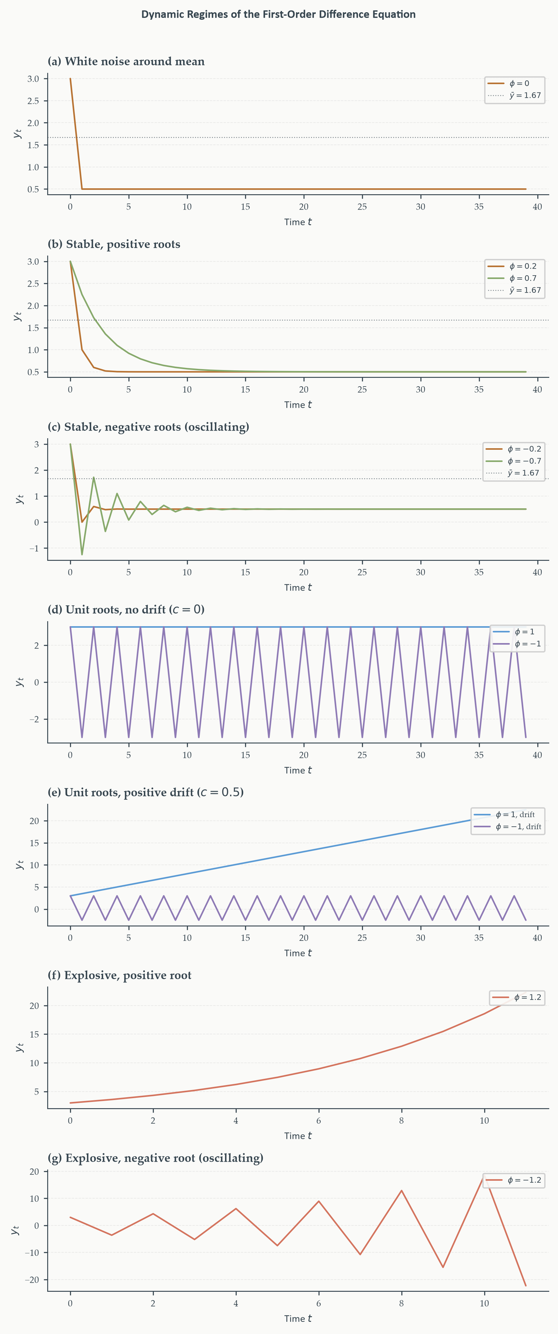
The figure below illustrates the different dynamic regimes for a range of characteristic roots. All stable paths share the long-run equilibrium $\bar{y} = 1.67$, and all paths begin at $y_0 = 3$ — a positive deviation from $\bar{y}$.
```{python}
#| label: fig-diffeq-paths
#| fig-cap: "Solution paths of the first-order difference equation $y_t = \\phi y_{t-1} + c$ for eight characteristic roots, all starting at $y_0 = 3$. Stable panels (a–c) show convergence to $\\bar{y} = 1.67$ (dotted line). Positive roots produce monotone paths; negative roots produce oscillation. Unit root paths (d) with $c=0$ wander without returning to any level; with $c=0.5$ (e) they trend linearly. Explosive paths (f–g) diverge rapidly; the negative explosive root produces amplifying oscillation."
#| fig-width: 6
#| fig-height: 14
#| code-fold: true
#| code-summary: "Show code — Figure 1.1"
T    = 40
y0   = 3.0
ybar = 1.67

def simulate(phi, c, y0=y0, T=T):
    y = np.zeros(T)
    y[0] = y0
    for i in range(1, T):
        y[i] = phi * y[i-1] + c
    return y

panels = [
    ([(0.0,  0.5,          r"$\phi=0$",         EO_COPPER)],
     "(a) White noise around mean", True),
    ([(0.2,  0.5*(1-0.2),  r"$\phi=0.2$",       EO_COPPER),
      (0.7,  0.5*(1-0.7),  r"$\phi=0.7$",       EO_SAGE)],
     "(b) Stable, positive roots", True),
    ([(-0.2, 0.5*(1+0.2),  r"$\phi=-0.2$",      EO_COPPER),
      (-0.7, 0.5*(1+0.7),  r"$\phi=-0.7$",      EO_SAGE)],
     "(c) Stable, negative roots (oscillating)", True),
    ([(1.0,  0.0,          r"$\phi=1$",          EO_SKYBLUE),
      (-1.0, 0.0,          r"$\phi=-1$",         EO_LAVENDER)],
     "(d) Unit roots, no drift ($c=0$)", False),
    ([(1.0,  0.5,          r"$\phi=1$, drift",   EO_SKYBLUE),
      (-1.0, 0.5,          r"$\phi=-1$, drift",  EO_LAVENDER)],
     r"(e) Unit roots, positive drift ($c=0.5$)", False),
    ([(1.2,  0.0,          r"$\phi=1.2$",        EO_TERRACOTTA)],
     "(f) Explosive, positive root", False),
    ([(-1.2, 0.0,          r"$\phi=-1.2$",       EO_TERRACOTTA)],
     "(g) Explosive, negative root (oscillating)", False),
]

T_exp = 12
fig, axes = plt.subplots(len(panels), 1, figsize=(6, 14))

for ax, (specs, title, show_ybar) in zip(axes, panels):
    is_exp = "(f)" in title or "(g)" in title
    T_use  = T_exp if is_exp else T
    t_use  = np.arange(T_use)
    for phi, c, lab, col in specs:
        y = simulate(phi, c, T=T_use)
        ax.plot(t_use, y, color=col, label=lab, linewidth=1.2)
    if show_ybar:
        ax.axhline(ybar, color=EO_CHARCOAL, linewidth=0.7,
                   linestyle=":", alpha=0.6, label=r"$\bar{y}=1.67$")
    ax.set_title(title)
    ax.set_xlabel("Time $t$")
    ax.set_ylabel("$y_t$")
    ax.legend(fontsize=6, loc="upper right")
    eo_style_ax(ax)

eo_suptitle(fig, "Dynamic Regimes of the First-Order Difference Equation")
fig.tight_layout()
plt.show()
```
Several features are worth noting. In panels (a) and (b), positive characteristic roots produce monotone convergence: the path moves smoothly toward $\bar{y}$ without overshooting. In panel (c), negative roots produce **oscillating convergence**: the path alternates above and below $\bar{y}$ while converging — a stylized representation of the kind of fluctuation we see in some economic series. Panels (d) and (e) show unit root behavior: without drift the path wanders aimlessly; with positive drift it trends steadily upward, never returning to any fixed level. Panels (f) and (g) show explosive behavior over a shorter horizon, illustrating how rapidly the process diverges when $|\phi| > 1$.
An important distinction: the oscillation produced by a **negative real root** in panel (c) and (g) alternates every single period — the sign of $y_t - \bar{y}$ flips at each step because $(-|\phi|)^t$ alternates in sign. This period-2 oscillation is the fastest possible. We will see shortly that **complex roots** produce smoother oscillations with longer periods, more representative of actual business cycles. The two mechanisms look superficially similar — both oscillate — but differ fundamentally in their period and in the functional form of the solution.
#### The Random Walk: A Special Case Worth Seeing
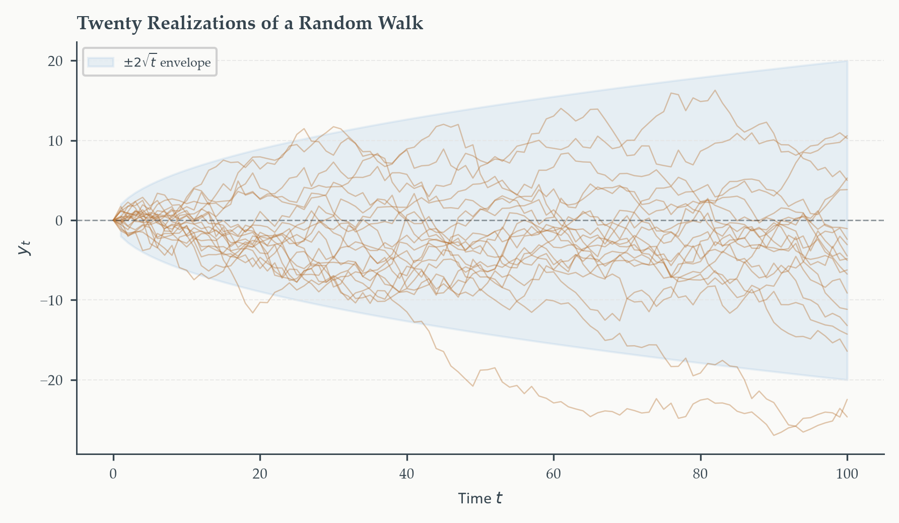
The pure [random walk](https://en.wikipedia.org/wiki/Random_walk) ($\phi = 1$, $c = 0$) deserves its own figure. Unlike any stable process, different realizations of a random walk fan out in completely different directions from the same starting point, and none of them returns to the initial level. The figure below simulates twenty independent random walk paths from the same starting value — the fan-shaped spreading is the visual signature of a unit root.
```{python}
#| label: fig-random-walk
#| fig-cap: "Twenty simulated random walk paths from the same starting value $y_0 = 0$. Each path is a single realization of $y_t = y_{t-1} + \\varepsilon_t$ with $\\varepsilon_t \\sim N(0,1)$. Unlike a stable process, the paths do not return to any fixed level — they spread out indefinitely. The grey band shows the theoretical $\\pm 2\\sqrt{t}$ envelope, confirming that the standard deviation grows as $\\sqrt{t}$."
#| fig-width: 6
#| fig-height: 3.5
#| code-fold: true
#| code-summary: "Show code — Figure 1.2"
rng = np.random.default_rng(seed=42)
T   = 100
N   = 20    # number of paths

fig, ax = plt.subplots(figsize=(6, 3.5))

for i in range(N):
    eps  = rng.normal(0, 1, T)
    path = np.cumsum(eps)
    path = np.insert(path, 0, 0)
    ax.plot(np.arange(T+1), path, color=EO_COPPER,
            linewidth=0.6, alpha=0.4)

# Theoretical +/- 2*sqrt(t) envelope
t_vec = np.arange(1, T+1)
ax.fill_between(t_vec,  2*np.sqrt(t_vec),
                        -2*np.sqrt(t_vec),
                color=EO_SKYBLUE, alpha=0.12,
                label=r"$\pm 2\sqrt{t}$ envelope")
ax.axhline(0, color=EO_CHARCOAL, linewidth=0.7,
           linestyle="--", alpha=0.5)
ax.set_title("Twenty Realizations of a Random Walk")
ax.set_xlabel("Time $t$")
ax.set_ylabel("$y_t$")
ax.legend(fontsize=6)
eo_style_ax(ax)
fig.tight_layout()
plt.show()
```
The grey band shows the theoretical $\pm 2\sqrt{t}$ envelope — the region within which each path falls with approximately 95% probability at each point in time. The envelope widens as $t$ grows, confirming the key property: $\text{Var}(y_t) = t\sigma^2$ grows linearly with time. No stable process has this property.
### Higher-Order Difference Equations, the Companion Matrix, and Eigenvalues {#sec-higher-order}
#### The $p$-th Order Case
A $p$-th order linear difference equation with a constant:
$$y_t = \phi_1 y_{t-1} + \phi_2 y_{t-2} + \cdots + \phi_p y_{t-p} + c \tag{1.4}$$
Using the lag operator: $\Phi(L)\,y_t = c$ where $\Phi(L) = 1 - \phi_1 L - \cdots - \phi_p L^p$. Adding white noise gives the **AR($p$) model**:
$$y_t = \phi_1 y_{t-1} + \cdots + \phi_p y_{t-p} + c + \varepsilon_t \tag{1.5}$$
The AR($p$) is the direct multiperiod generalization of the AR(1): the current value depends on the previous $p$ periods, each with its own coefficient.
#### The Companion Matrix Representation
A key insight — connecting difference equations to linear algebra — is that any $p$-th order scalar difference equation can be rewritten as a **first-order vector difference equation** by stacking the relevant lags into a state vector.
Define the $p$-dimensional state vector $\mathbf{z}_t = (y_t,\, y_{t-1},\, \ldots,\, y_{t-p+1})'$. Then equation (1.4) can be written as:
$$\mathbf{z}_t = \mathbf{F}\mathbf{z}_{t-1} + \mathbf{c} \tag{1.6}$$
where $\mathbf{F}$ is the $p \times p$ **companion matrix**:
$$\mathbf{F} = \begin{pmatrix}
\phi_1 & \phi_2 & \phi_3 & \cdots & \phi_{p-1} & \phi_p \\
1 & 0 & 0 & \cdots & 0 & 0 \\
0 & 1 & 0 & \cdots & 0 & 0 \\
\vdots & & \ddots & & & \vdots \\
0 & 0 & 0 & \cdots & 1 & 0
\end{pmatrix}$$
and $\mathbf{c} = (c, 0, 0, \ldots, 0)'$. The companion matrix has the AR coefficients in its first row, and an identity submatrix in the remaining rows that simply records that $y_{t-j} = y_{t-j}$.
To verify: reading the first row of (1.6) gives $y_t = \phi_1 y_{t-1} + \phi_2 y_{t-2} + \cdots + \phi_p y_{t-p} + c$ — exactly equation (1.4). Reading the second row gives $y_{t-1} = y_{t-1}$ — trivially true. The companion matrix representation is not a new equation; it is the original $p$-th order equation reorganized.
#### Eigenvalues and Stability
The solution of the first-order vector system (1.6) depends on the powers of $\mathbf{F}$: iterating backwards, $\mathbf{z}_t = \mathbf{F}^t \mathbf{z}_0 + \sum_{s=0}^{t-1}\mathbf{F}^s \mathbf{c}$. The behavior of $\mathbf{F}^t$ as $t \to \infty$ is determined by the **[eigenvalues](https://en.wikipedia.org/wiki/Eigenvalues_and_eigenvectors) of $\mathbf{F}$** — the values $\lambda$ satisfying $\det(\mathbf{F} - \lambda \mathbf{I}) = 0$. Recall from linear algebra that eigenvalues are the scalars by which a matrix stretches or contracts its eigenvectors; when we raise a matrix to a power $t$, the eigenvalues are raised to that same power $\lambda^t$, so their moduli determine whether the system grows, decays, or oscillates as $t$ increases.
A fundamental result of linear algebra connects the eigenvalues of $\mathbf{F}$ directly to the characteristic roots of the original scalar equation:
::: {.callout-note}
## Proposition 1.1 — Eigenvalues of the Companion Matrix
The eigenvalues of the companion matrix $\mathbf{F}$ are identical to the characteristic roots $\lambda_1, \lambda_2, \ldots, \lambda_p$ of the $p$-th order difference equation (1.4).
:::
To see why, note that the characteristic polynomial of $\mathbf{F}$ — the polynomial whose roots are its eigenvalues — is:
$$\det(\lambda\mathbf{I} - \mathbf{F}) = \lambda^p - \phi_1\lambda^{p-1} - \phi_2\lambda^{p-2} - \cdots - \phi_p$$
which is exactly the characteristic equation of the scalar difference equation. The eigenvalues of $\mathbf{F}$ and the characteristic roots of (1.4) are the same objects.
This connection is not merely algebraic — it is conceptually important. It means the stability of a time series process can be analyzed entirely through the eigenvalues of its companion matrix, a standard object in linear algebra. For an AR(2) with $p = 2$, for example:
$$\mathbf{F} = \begin{pmatrix} \phi_1 & \phi_2 \\ 1 & 0 \end{pmatrix}$$
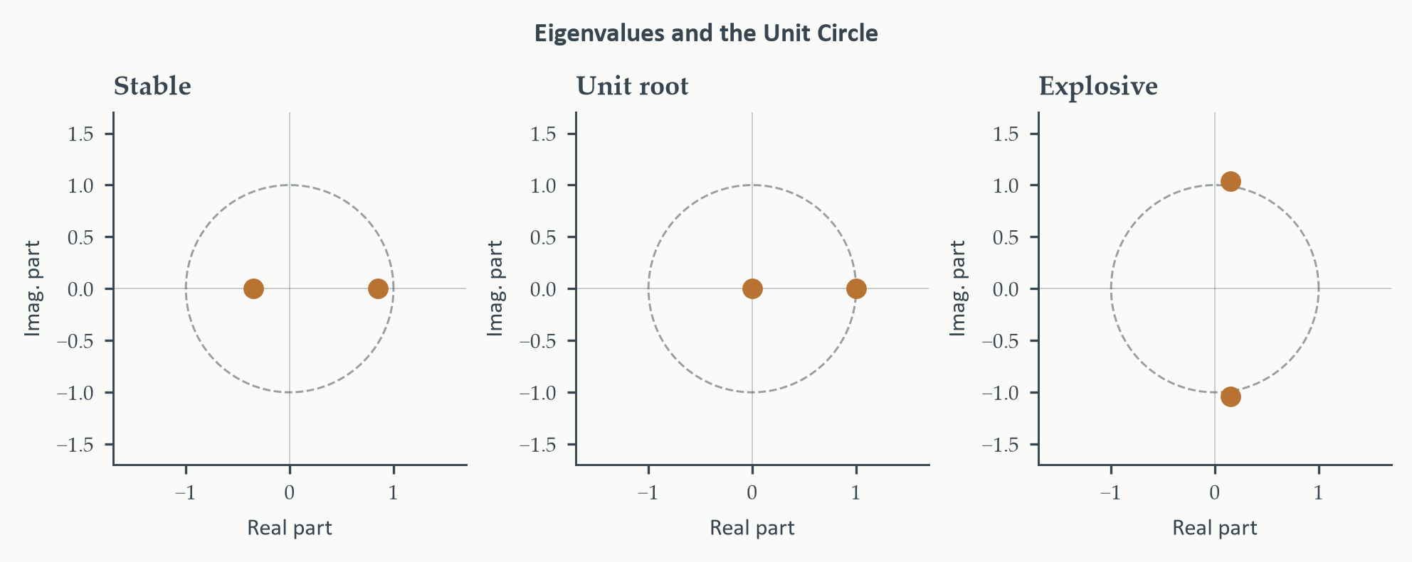
The eigenvalues are the two roots of $\lambda^2 - \phi_1\lambda - \phi_2 = 0$ — precisely the characteristic equation. Whether these eigenvalues lie inside, on, or outside the unit circle determines whether the AR(2) process is stable, has a unit root, or is explosive.
::: {.callout-note}
## Definition 1.5 — Stability of a $p$-th Order Difference Equation
The equation (1.4) — equivalently, the AR($p$) model (1.5) — is **stable** if and only if all $p$ eigenvalues of the companion matrix $\mathbf{F}$ satisfy $|\lambda_j| < 1$. Equivalently, all roots of the characteristic polynomial $\lambda^p - \phi_1\lambda^{p-1} - \cdots - \phi_p = 0$ lie strictly inside the unit circle.
If any eigenvalue has $|\lambda_j| = 1$, the system has a unit root. If any eigenvalue has $|\lambda_j| > 1$, the system is explosive.
:::
The general homogeneous solution, when all eigenvalues are distinct, is:
$$y_t^{(h)} = A_1\lambda_1^t + A_2\lambda_2^t + \cdots + A_p\lambda_p^t$$
where $A_1, \ldots, A_p$ are determined by $p$ initial conditions. The particular solution for a constant forcing term, when no eigenvalue equals 1, is:
$$\bar{y} = \frac{c}{1 - \phi_1 - \phi_2 - \cdots - \phi_p} = \frac{c}{\Phi(1)}$$
::: {.callout-warning}
## Two Equivalent Stationarity Conventions
In terms of the **characteristic equation**: all eigenvalues satisfy $|\lambda_j| < 1$ (inside the unit circle). In terms of the **lag polynomial** $\Phi(z) = 1 - \phi_1 z - \cdots - \phi_p z^p$: all roots of $\Phi(z) = 0$ satisfy $|z_j| > 1$ (outside the unit circle). These are equivalent because the roots of $\Phi(z)$ are the reciprocals of the eigenvalues.
:::
#### Real vs. Complex Eigenvalues and Oscillatory Behavior
When all eigenvalues are real, the solution path is monotone (positive eigenvalue) or alternating in sign (negative eigenvalue) at each period, as we saw in the first-order case. When eigenvalues are **complex** — always occurring in conjugate pairs $\lambda, \bar{\lambda} = re^{\pm i\omega}$ for equations with real coefficients — the solution exhibits oscillatory behavior of a different and richer kind.
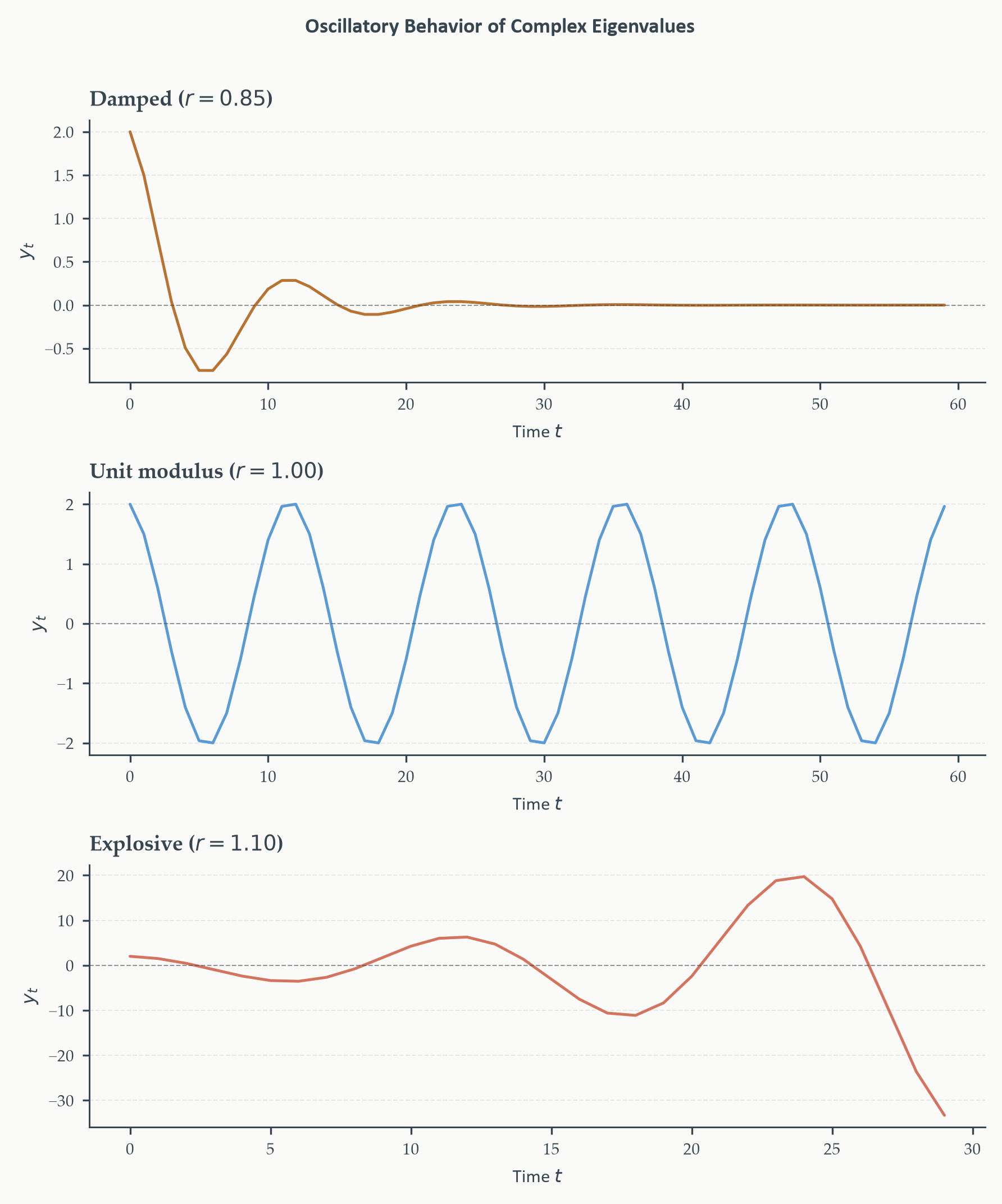
To understand this intuitively, a complex eigenvalue pair encodes two pieces of information simultaneously: how quickly the oscillation decays or grows (the **modulus** $r = |\lambda|$) and how fast the oscillation cycles (the **argument** $\omega$). The contribution of a complex conjugate pair to the solution is a **damped sinusoid**:
$$A\,r^t\cos(\omega t + \theta)$$
where $A$ and $\theta$ are determined by initial conditions. The modulus $r$ is the envelope:
- When $r < 1$: the amplitude $r^t$ shrinks — a **damped oscillation** that gradually returns to the long-run level. This is the pattern associated with stable business cycle dynamics.
- When $r = 1$: a **sustained oscillation** that neither grows nor decays.
- When $r > 1$: an **amplifying oscillation** — explosive in the oscillatory sense.
The argument $\omega$ (in radians per period) determines the **period** of the cycle: $P = 2\pi/\omega$ periods to complete one full oscillation. A complex eigenvalue pair with $\omega = \pi/6$ and quarterly data implies a cycle period of $P = 2\pi/(\pi/6) = 12$ quarters — a three-year cycle, squarely in the range of typical business cycle frequencies.
**This is the key distinction from negative real eigenvalues.** A negative real eigenvalue $\lambda < 0$ produces oscillation that alternates every single period: $\lambda^t$ changes sign at each step because $(-|\lambda|)^t$ alternates. This is period-2 oscillation — the fastest possible, completing a full cycle in just two periods. Complex eigenvalues, by contrast, allow any period $P = 2\pi/\omega \geq 2$. Real economies exhibit business cycles with periods of 6–32 quarters — far too slow to be explained by negative real eigenvalues, but naturally produced by complex conjugate pairs with appropriate arguments. The oscillatory behavior of complex roots is therefore not just a mathematical curiosity; it is one of the mechanisms through which business-cycle-like dynamics arise in AR($p$) models.
```{python}
#| label: fig-complex-roots
#| fig-cap: "AR(2) solution paths for complex eigenvalues with the same argument $\\omega = \\pi/6$ (twelve-period cycle, three years of quarterly data) but different moduli. The damped case ($r=0.85$, copper) oscillates and converges. The unit-modulus case ($r=1.0$, blue) sustains the oscillation indefinitely. The explosive case ($r=1.1$, terracotta) shows growing oscillations. Note the smooth sinusoidal shape — quite different from the period-2 alternation produced by negative real eigenvalues."
#| fig-width: 6
#| fig-height: 7
#| code-fold: true
#| code-summary: "Show code — Figure 1.3"
def ar2_from_complex_roots(r, omega, T=60, y0=2.0, y1=1.5):
    phi1 =  2 * r * np.cos(omega)
    phi2 = -r ** 2
    y    = np.zeros(T)
    y[0] = y0
    y[1] = y1
    for t in range(2, T):
        y[t] = phi1 * y[t-1] + phi2 * y[t-2]
    return y

omega  = np.pi / 6
specs  = [(0.85, EO_COPPER,     r"Damped ($r=0.85$)",         60),
          (1.00, EO_SKYBLUE,    r"Unit modulus ($r=1.00$)",   60),
          (1.10, EO_TERRACOTTA, r"Explosive ($r=1.10$)",      30)]

fig, axes = plt.subplots(3, 1, figsize=(6, 7))

for ax, (r, col, lab, T_use) in zip(axes, specs):
    y = ar2_from_complex_roots(r, omega, T=T_use)
    ax.plot(np.arange(T_use), y, color=col, linewidth=1.2, label=lab)
    ax.axhline(0, color=EO_CHARCOAL, linewidth=0.5,
               linestyle="--", alpha=0.5)
    ax.set_title(lab)
    ax.set_xlabel("Time $t$")
    ax.set_ylabel("$y_t$")
    eo_style_ax(ax)

eo_suptitle(fig, "Oscillatory Behavior of Complex Eigenvalues")
fig.tight_layout()
plt.show()
```
#### Root Diagrams
A convenient visual summary of the stability condition plots the eigenvalues in the complex plane with the unit circle as a reference. All eigenvalues inside the circle — stable. Any eigenvalue on the circle — unit root. Any eigenvalue outside — explosive.
```{python}
#| label: fig-root-diagrams
#| fig-cap: "Eigenvalue diagrams for three AR(2) specifications. Left: both roots inside the unit circle — stable, stationary process ($\\phi_1=0.5$, $\\phi_2=0.3$; roots at $0.85$ and $-0.35$). Center: one root exactly on the circle — unit root ($\\phi_1=1.0$, $\\phi_2=0.0$; roots at $1.0$ and $0.0$). Right: both complex roots outside the unit circle — explosive process ($\\phi_1=0.3$, $\\phi_2=-1.1$; complex conjugate pair with modulus $1.05$)."
#| fig-width: 6
#| fig-height: 2.8
#| code-fold: true
#| code-summary: "Show code — Figure 1.4"
def char_roots_ar2(phi1, phi2):
    return np.roots([1, -phi1, -phi2])

specs_rd = [
    (0.5,  0.3,   "Stable"),
    (1.0,  0.0,   "Unit root"),
    (0.3, -1.1,   "Explosive"),
]

fig, axes = plt.subplots(1, 3, figsize=(6.5, 2.5), constrained_layout=True)
theta = np.linspace(0, 2*np.pi, 300)

for ax, (phi1, phi2, title) in zip(axes, specs_rd):
    roots = char_roots_ar2(phi1, phi2)
    ax.plot(np.cos(theta), np.sin(theta),
            color=EO_CHARCOAL, linewidth=0.7, linestyle="--", alpha=0.5)
    ax.axhline(0, color=EO_CHARCOAL, linewidth=0.4, alpha=0.3)
    ax.axvline(0, color=EO_CHARCOAL, linewidth=0.4, alpha=0.3)
    for root in roots:
        ax.scatter(root.real, root.imag,
                   color=EO_COPPER, s=35, zorder=5)
    ax.set_xlim(-1.7, 1.7)
    ax.set_ylim(-1.7, 1.7)
    ax.set_aspect("equal")
    ax.set_title(title)
    ax.set_xlabel("Real part")
    ax.set_ylabel("Imag. part")
    ax.grid(False)
    eo_style_ax(ax)

eo_suptitle(fig, "Eigenvalues and the Unit Circle")
plt.show()
```
## The ACF and PACF {#sec-acfpacf}
### Measuring Temporal Dependence
Stationarity, as we will define it formally in the next section, is the condition that a process has a stable probabilistic structure over time. But before developing that formal definition, it is useful to have the tools to describe and measure what temporal dependence actually looks like in practice. Two processes can both be stationary while having very different patterns of dependence: one nearly uncorrelated from one period to the next, another remaining strongly correlated for many lags. The tools in this section let us characterize those patterns — and they will serve as our primary informal diagnostic for nonstationarity before we introduce formal tests.
### The Autocovariance and Autocorrelation Functions
For a weakly stationary process $\{y_t\}$ with mean $\mu$, the **autocovariance function** (ACVF) at lag $h$ is:
$$\gamma(h) = \text{Cov}(y_t, y_{t-h}) = \mathbb{E}[(y_t - \mu)(y_{t-h} - \mu)]$$
By weak stationarity, this depends only on $h$, not on $t$. Three properties follow immediately: **symmetry** ($\gamma(h) = \gamma(-h)$), **maximum at zero** ($|\gamma(h)| \leq \gamma(0) = \sigma^2$, from Cauchy-Schwarz), and **positive semidefiniteness** (the ACVF matrix is positive semidefinite — not every function can be an autocovariance function).
Normalizing by the variance gives the **autocorrelation function** (ACF):
$$\rho(h) = \frac{\gamma(h)}{\gamma(0)}, \qquad \rho(0) = 1, \quad |\rho(h)| \leq 1$$
The sample ACF is estimated by:
$$\hat{\rho}(h) = \frac{\hat{\gamma}(h)}{\hat{\gamma}(0)}, \qquad \hat{\gamma}(h) = \frac{1}{T}\sum_{t=h+1}^{T}(y_t - \bar{y})(y_{t-h} - \bar{y})$$
The divisor is $T$ rather than $T-h$ to ensure positive semidefiniteness of the sample ACVF matrix. Under the null that the series is white noise, $\hat{\rho}(h) \overset{a}{\sim} N(0, 1/T)$ for large $T$, giving the standard 95% confidence bands at $\pm 1.96/\sqrt{T}$ in ACF plots.
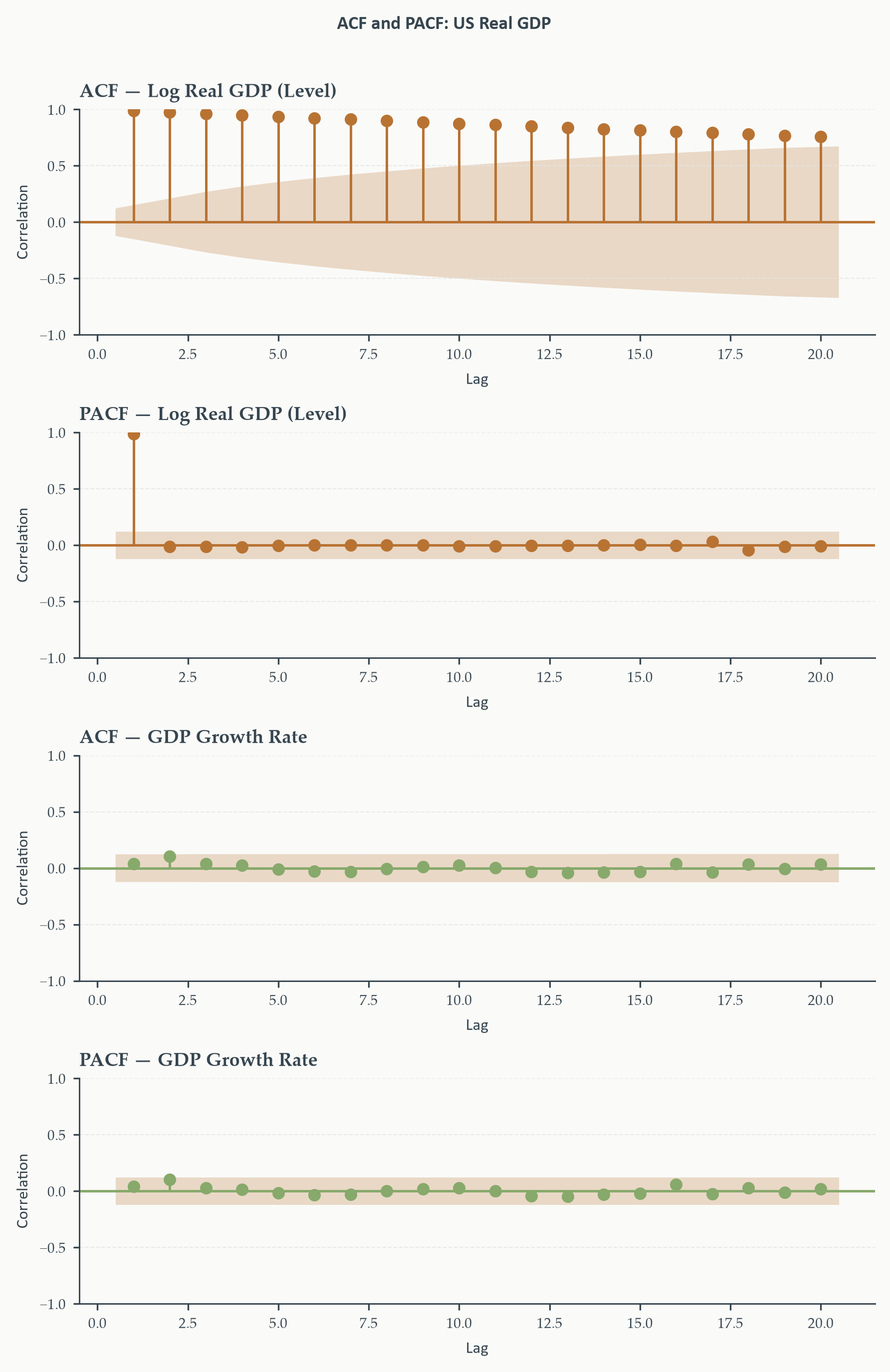
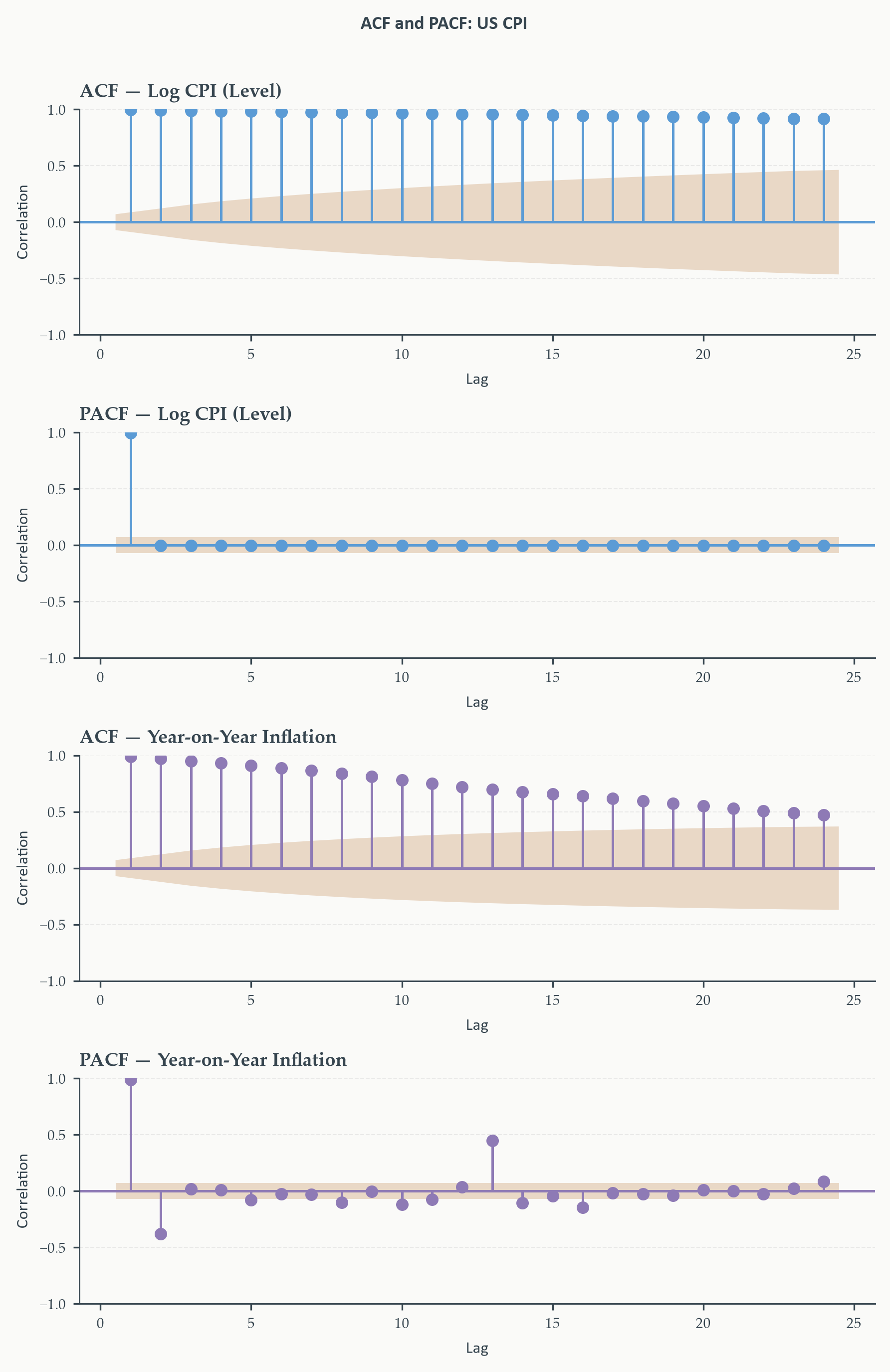
The shape of the ACF immediately reveals temporal structure. A **slowly decaying ACF** — remaining close to 1.0 across many lags — is the visual fingerprint of a unit root process. A **geometrically decaying ACF** — dropping steadily toward zero — suggests an autoregressive process. An ACF that **cuts off sharply** after a small number of lags suggests a moving average process. An ACF **indistinguishable from zero** at all nonzero lags is the signature of white noise. We will connect these patterns to specific model classes in Chapter 3.
### The Partial Autocorrelation Function
The ACF measures total correlation between $y_t$ and $y_{t-h}$, including indirect effects transmitted through intermediate lags. The **partial autocorrelation function** (PACF) isolates the direct effect, after removing the linear influence of all intervening observations.
The PACF at lag $h$, denoted $\alpha(h)$, is the coefficient on $y_{t-h}$ in the OLS regression of $y_t$ on its $h$ most recent lags:
$$y_t = \phi_{h,1}y_{t-1} + \cdots + \phi_{h,h}y_{t-h} + \varepsilon_t^{(h)}, \qquad \alpha(h) = \phi_{h,h}$$
At lag 1, there is nothing to partial out: $\alpha(1) = \rho(1)$. At lag 2:
$$\alpha(2) = \frac{\rho(2) - \rho(1)^2}{1 - \rho(1)^2}$$
For general $h$, the PACF is computed via the Yule-Walker equationsWe derive this recursion properly in Chapter 3, where it appears in its natural context as a method for estimating AR(p) parameters. For now, the key skill is interpreting the output, not computing it by hand.
The ACF and PACF together serve as the primary diagnostic tool for model identification. Their joint behavior reveals the structure of the underlying process and guides the choice of model class and order. Chapter 3 develops these identification patterns in full, once the AR, MA, and ARMA families have been formally introduced. For now, the key skill is computing and reading these functions — the interpretation deepens with each model class we study.
### Python Example: ACF and PACF for US GDP and CPI
```{python}
#| label: fig-acfpacf-gdp
#| fig-cap: "ACF and PACF for US real GDP. Top two panels: log level. Bottom two panels: QoQ growth rate. The log-level ACF decays extremely slowly — barely moving from 1.0 across twenty lags — the visual fingerprint of an integrated $I(1)$ process. After log-differencing, the ACF drops sharply and the PACF shows one dominant spike at lag 1. The interpretation of these patterns in terms of specific AR, MA, and ARMA models is developed in Chapter 3."
#| fig-width: 6
#| fig-height: 9
#| code-fold: true
#| code-summary: "Show code — Figure 1.5"
fig, axes = plt.subplots(4, 1, figsize=(6, 9))

plot_acf(gdp["Log Real GDP"].dropna(), lags=20, ax=axes[0],
         color=EO_COPPER, vlines_kwargs={"colors": EO_COPPER},
         title="ACF — Log Real GDP (Level)", zero=False, alpha=0.05)

plot_pacf(gdp["Log Real GDP"].dropna(), lags=20, ax=axes[1],
          color=EO_COPPER, vlines_kwargs={"colors": EO_COPPER},
          method="ywm", title="PACF — Log Real GDP (Level)",
          zero=False, alpha=0.05)

plot_acf(gdp["GDP Growth (QoQ)"].dropna(), lags=20, ax=axes[2],
         color=EO_SAGE, vlines_kwargs={"colors": EO_SAGE},
         title="ACF — GDP Growth Rate", zero=False, alpha=0.05)

plot_pacf(gdp["GDP Growth (QoQ)"].dropna(), lags=20, ax=axes[3],
          color=EO_SAGE, vlines_kwargs={"colors": EO_SAGE},
          method="ywm", title="PACF — GDP Growth Rate",
          zero=False, alpha=0.05)

for ax in axes:
    ax.set_xlabel("Lag")
    ax.set_ylabel("Correlation")
    eo_style_ax(ax)
    for line in ax.lines:
        if line.get_linestyle() == "--":
            line.set_color(EO_TERRACOTTA)
            line.set_linewidth(0.7)

eo_suptitle(fig, "ACF and PACF: US Real GDP")
fig.tight_layout()
plt.show()
```
```{python}
#| label: fig-acfpacf-cpi
#| fig-cap: "ACF and PACF for US CPI. Top two panels: log level. Bottom two panels: year-on-year inflation. The log-level CPI has a near-unit ACF — clearly nonstationary. The inflation series shows richer autocorrelation structure than GDP growth: the ACF decays slowly and remains significant at many lags, while the PACF drops after a few lags. This persistence reflects, in part, the regime-dependence of inflation dynamics discussed below."
#| fig-width: 6
#| fig-height: 9
#| code-fold: true
#| code-summary: "Show code — Figure 1.6"
fig, axes = plt.subplots(4, 1, figsize=(6, 9))

plot_acf(cpi["Log CPI"].dropna(), lags=24, ax=axes[0],
         color=EO_SKYBLUE, vlines_kwargs={"colors": EO_SKYBLUE},
         title="ACF — Log CPI (Level)", zero=False, alpha=0.05)

plot_pacf(cpi["Log CPI"].dropna(), lags=24, ax=axes[1],
          color=EO_SKYBLUE, vlines_kwargs={"colors": EO_SKYBLUE},
          method="ywm", title="PACF — Log CPI (Level)",
          zero=False, alpha=0.05)

plot_acf(cpi["Inflation (YoY)"].dropna(), lags=24, ax=axes[2],
         color=EO_LAVENDER, vlines_kwargs={"colors": EO_LAVENDER},
         title="ACF — Year-on-Year Inflation", zero=False, alpha=0.05)

plot_pacf(cpi["Inflation (YoY)"].dropna(), lags=24, ax=axes[3],
          color=EO_LAVENDER, vlines_kwargs={"colors": EO_LAVENDER},
          method="ywm", title="PACF — Year-on-Year Inflation",
          zero=False, alpha=0.05)

for ax in axes:
    ax.set_xlabel("Lag")
    ax.set_ylabel("Correlation")
    eo_style_ax(ax)
    for line in ax.lines:
        if line.get_linestyle() == "--":
            line.set_color(EO_TERRACOTTA)
            line.set_linewidth(0.7)

eo_suptitle(fig, "ACF and PACF: US CPI")
fig.tight_layout()
plt.show()
```
## Stationarity {#sec-stationarity}
The mathematics of the difference equations section revealed something fundamental: the behavior of a time series process — whether its past influences decay, persist, or explode — depends on where the eigenvalues of its companion matrix sit relative to the unit circle. The ACF and PACF tools just introduced gave us a way to see this dependence structure empirically. The statistical concept of stationarity now translates both of these insights into the language of probability.
[Stationarity](https://en.wikipedia.org/wiki/Stationary_process) is the condition that a process has a stable probabilistic structure over time. Not that it is constant — economic time series fluctuate continuously — but that the statistical properties governing those fluctuations do not themselves change. A stationary process today has, in a precise sense, the same distribution it had yesterday and will have tomorrow. This stability is what makes it possible to estimate parameters from a single observed history and trust that those parameters remain relevant for the future.
When stationarity fails, the usual machinery of statistical inference breaks down in several ways. Estimators may not converge to their population values. Standard errors may be wrong. Test statistics may follow non-standard distributions, rendering conventional inference invalid. Most practically, a model fitted to one part of the data may say nothing useful about another. The **spurious regression problem** — two completely unrelated nonstationary series appearing strongly correlated simply because both trend in the same direction — is perhaps the most well-known consequence, and it is one of the most dangerous traps in applied econometrics.
### Strict and Weak Stationarity
::: {.callout-note}
## Definition 1.6 — Strict Stationarity
A stochastic process $\{y_t\}$ is **strictly stationary** if, for any finite collection of time indices $t_1 < t_2 < \cdots < t_k$ and any integer $h$, the joint distribution of $(y_{t_1}, \ldots, y_{t_k})$ is identical to the joint distribution of $(y_{t_1+h}, \ldots, y_{t_k+h})$.
:::
Strict stationarity says that shifting the entire process by any number of periods changes nothing about its distribution — not means, not variances, not shapes, not tails. This is an extremely strong condition, rarely verified directly. In practice we rely on a weaker but more tractable definition.
::: {.callout-note}
## Definition 1.7 — Weak (Covariance) Stationarity
A stochastic process $\{y_t\}$ is **weakly stationary** (or **covariance stationary**) if:
1. $\mathbb{E}[y_t] = \mu < \infty$ for all $t$ — the mean is finite and constant over time.
2. $\text{Var}(y_t) = \sigma^2 < \infty$ for all $t$ — the variance is finite and constant over time.
3. $\text{Cov}(y_t, y_{t-h}) = \gamma(h)$ for all $t$ and all $h$ — the covariance between any two observations depends only on the lag $h$, not on when in time they occur.
:::
**Condition 1** rules out trending means. A series whose average level grows over time — like the level of nominal GDP — fails this condition immediately.
**Condition 2** rules out changing variance. As we saw in the random walk figure, $\text{Var}(y_t)$ grows linearly with $t$ for a unit root process — a direct violation.
**Condition 3** is the subtlest. It says the covariance structure depends only on distance in time, not on location in time. The covariance between GDP growth in 1995Q1 and 1995Q2 should equal the covariance between GDP growth in 2010Q1 and 2010Q2 — both pairs are one quarter apart. This is what makes the autocovariance function $\gamma(h)$ a well-defined, estimable object: we pool all pairs of observations separated by lag $h$, regardless of when they occur, to estimate a single number.
The relationship between the two definitions: strict stationarity with finite variance implies weak stationarity. The converse is false in general. The important exception is **Gaussian processes** — because the normal distribution is fully characterized by its first two moments, a weakly stationary Gaussian process is automatically strictly stationary. Weak stationarity is the operative assumption throughout this course.
### Types of Non-Stationarity {#sec-nonstationarity}
Not all non-stationarity is the same, and the type matters for how we handle it. There are three main forms in economic data.
#### Trend Stationarity
A process is **[trend stationary](https://en.wikipedia.org/wiki/Trend-stationary_process)** if it fluctuates around a deterministic trend — a fixed function of time — with stationary fluctuations:
$$y_t = \alpha + \beta t + \varepsilon_t$$
where $u_t$ is weakly stationary. The series $y_t$ is nonstationary because $\mathbb{E}[y_t] = \alpha + \beta t$ depends on $t$. But the deviations from trend are stationary. Crucially, a shock that perturbs $u_t$ at time $t$ has only a **transitory** effect: the series eventually returns to the deterministic trend path. To achieve stationarity, we **detrend** — regress $y_t$ on a constant and time and work with the residuals.
#### Difference Stationarity and Unit Roots
A process is **difference stationary** if it is nonstationary in levels but stationary after first differencing — arising when the characteristic polynomial has a root on the unit circle. The canonical example is the random walk with drift:
$$y_t = c + y_{t-1} + \varepsilon_t$$
First differencing gives $\Delta y_t = c + \varepsilon_t$, which is stationary. But the level is not: its variance grows without bound, and unlike the trend-stationary case, shocks are **permanent** — a positive $\varepsilon_t$ raises $y_t$ permanently above the path it would otherwise have followed.
The distinction between transitory and permanent shocks has profound economic implications. Is an unexpected recession a transitory deviation from a stable growth path, or a permanent downward shift in the level of output? The answer changes the interpretation of business cycles, the conduct of policy, and the specification of macroeconometric models.
A series requiring $d$ rounds of differencing to achieve stationarity is **integrated of order $d$**, written $I(d)$. Most economic level series are $I(1)$.
#### Explosive Processes
When any eigenvalue has modulus strictly greater than 1, the process is **explosive**: deviations grow without bound. Explosive processes are rare in economic data over long horizons, but arise in specific contexts — asset price bubbles being the most prominent example. Detecting such episodes is an active research area that builds directly on the methods developed here.
::: {.callout-note}
### Summary: Types of Non-Stationarity
| Type | Source | Shocks | Fix |
|-----------------------|------------------------------------------------|------------|-------------------|
| Trend stationar y | Deterministic trend | Transitory | Detrend |
| Difference stationary | Unit root ($|\lambda|=1$) | Permanent | First difference |
| Explosive | Eigenvalue outside unit circle ($|\lambda|>1$) | Amplifying | Specialized tests |
: Three types of non-stationarity and their treatments {#tbl-nonstationarity}
:::
## Assessing and Addressing Non-Stationarity {#sec-unitroots}
Before reaching for a formal statistical test, the first step in assessing stationarity is always visual inspection. A well-constructed time plot reveals most of what we need to know.
A **trend-stationary** series shows a clear upward or downward drift, but fluctuations around that drift appear roughly constant in amplitude. A straight line through the data looks like a reasonable fit.
A **difference-stationary** (unit root) series wanders without apparent direction. There is no deterministic path the data seem to track. The series drifts up for a while, then drifts back down, with no tendency to return to a fixed level. The variance appears to grow with time — consistent with what we showed analytically for the random walk.
An **explosive** series accelerates: the rate of change increases over time, and the series leaves any reference path behind at increasing speed.
Looking at the **sample ACF** provides a further informal diagnostic. A stationary series has an ACF that decays reasonably quickly toward zero. A unit root series has an ACF that decays extremely slowly — often remaining close to 1.0 for many lags — exactly as we saw in the figures above for log GDP and log CPI. These visual tools are informative but imprecise. For formal inference, we need the ADF and KPSS tests.
### The Augmented Dickey-Fuller Test {#sec-adf}
#### The Regression Framework
The [ADF test](https://en.wikipedia.org/wiki/Dickey%E2%80%93Fuller_test) builds directly on the AR(1) regression framework derived in the difference equations section. Recall that $y_t = \phi y_{t-1} + c + \varepsilon_t$ can be rewritten as:
$$\Delta y_t = \delta y_{t-1} + c + \varepsilon_t, \qquad \delta = \phi - 1$$
The unit root null $\phi = 1$ becomes $H_0: \delta = 0$; the stationary alternative $\phi < 1$ becomes $H_1: \delta < 0$. This is a one-sided test. The **Augmented Dickey-Fuller test** adds lagged differences to absorb serial correlation in the errors:
$$\Delta y_t = \delta y_{t-1} + \sum_{j=1}^{p} \psi_j \Delta y_{t-j} + c + \beta t + \varepsilon_t \tag{1.7}$$
The test statistic is the $t$-ratio on $\hat{\delta}$. Three specifications correspond to different assumptions about deterministic components:
| Specification | Regression equation | Use when... |
|:---|:---|:---|
| No constant, no trend | $\Delta y_t = \delta y_{t-1} + \sum_{j=1}^{p}\psi_j\Delta y_{t-j} + \varepsilon_t$ | Series is zero-mean with no drift |
| Constant only | $\Delta y_t = c + \delta y_{t-1} + \sum_{j=1}^{p}\psi_j\Delta y_{t-j} + \varepsilon_t$ | Series has a non-zero mean |
| Constant and trend | $\Delta y_t = c + \beta t + \delta y_{t-1} + \sum_{j=1}^{p}\psi_j\Delta y_{t-j} + \varepsilon_t$ | Series may trend under $H_1$ |
: ADF specification choices {#tbl-adf-specs}
Always inspect the time plot before choosing. Including a trend when none is present reduces power; omitting a constant when one exists distorts size.
#### Non-Standard Critical Values
Under $H_0$, $y_{t-1}$ is an integrated process, so $\hat{\delta}$ does not follow a standard $t$-distribution — it follows the left-skewed **Dickey-Fuller distribution**, with more mass in its left tail than the normal. Using standard critical values would cause severe under-rejection of the unit root null. The correct critical values were tabulated by [Dickey and Fuller (1979)](https://www.jstor.org/stable/2286348) and are built into all standard software.
#### Choosing the Lag Length
**Information criteria.** Before covering information criteria formally — that requires introducing likelihood, which we do in a later chapter — the basic idea is intuitive. More lags always improve in-sample fit, but adding lags that carry no real information makes the test noisier. Information criteria formalize this tradeoff by penalizing complexity. The AIC and BIC take the form "measure of fit minus penalty for complexity":
$$\text{AIC}(p) = \log\hat{\sigma}^2_p + \frac{2(p+k)}{T} \qquad \text{BIC}(p) = \log\hat{\sigma}^2_p + \frac{\log(T)(p+k)}{T}$$
where $\hat{\sigma}^2_p$ is the estimated residual variance and $k$ counts the deterministic terms. BIC penalizes additional lags more heavily than AIC and tends to select more parsimonious models. We select the $p$ that minimizes the chosen criterion. The full technical treatment — why these specific penalty terms, how they relate to likelihood, and their asymptotic properties — is developed in the model selection chapter.
**General-to-specific (GETS).** Start with $p_{\max} = \lfloor 12(T/100)^{1/4} \rfloor$ (the Schwert rule). Test whether the last lag $\psi_p$ is statistically significant. If not, drop it and test $\psi_{p-1}$, continuing until a significant lag is found or $p = 0$.
#### Interpreting the Output
The ADF test produces three things: a **test statistic** (always negative; more negative means stronger evidence against the unit root null), a **p-value** (below 0.05 leads to rejection at the 5% level), and **critical values** at 1%, 5%, and 10%.
::: {.callout-warning}
### Two Common Mistakes
**Mistake 1: Failing to reject is not evidence of a unit root.** The ADF has low power against near-unit-root alternatives. A large p-value means the data are insufficient to reject the null, not that the null is true.
**Mistake 2: The specification matters.** Always let the visual appearance of the data guide the choice of deterministic terms.
:::
### The KPSS Test {#sec-kpss}
#### Reversing the Null
The ADF test is conservative about rejecting unit roots — by design, since it controls the probability of falsely declaring a unit root series stationary. A near-unit-root series may routinely survive the ADF test. The **[KPSS test](https://en.wikipedia.org/wiki/KPSS_test)** (Kwiatkowski, Phillips, Schmidt, and Shin, 1992) addresses this by reversing the null: stationarity is the null, a unit root is the alternative. Running both tests together provides evidence that neither test alone can supply.
#### The Regression Framework
The KPSS test decomposes the series as:
$$y_t = \beta t + r_t + \varepsilon_t$$
where $\beta t$ is a deterministic trend, $\varepsilon_t$ is a stationary error, and $r_t = r_{t-1} + u_t$ is a random walk with $u_t \sim WN(0,\sigma_u^2)$. The null $\sigma_u^2 = 0$ means the random walk component is absent — the series is stationary around its deterministic part. The alternative $\sigma_u^2 > 0$ allows a unit root.
The two stochastic components play very different roles, and keeping them conceptually separate is the key to understanding the test. The component $r_t$ is the **object under scrutiny**: it is the stochastic trend whose variance $\sigma_u^2$ the test is trying to detect. Under the null, $\sigma_u^2 = 0$ so $u_t \equiv 0$ and $r_t = r_0$ for all $t$ — a constant that simply shifts the level of the series. Under the alternative, $r_t$ wanders without bound, and this wandering is what makes the series nonstationary.
The component $\varepsilon_t$, by contrast, is the **legitimate stationary variation** in the series — the part that fluctuates around the deterministic trend even when no unit root is present. Crucially, $\varepsilon_t$ is allowed to be serially correlated: a stationary but persistent process will fluctuate for extended periods without returning to its mean, and it would be wrong to mistake that persistence for a unit root. This is exactly why the long-run variance estimator $\hat{\lambda}^2$ is needed: it corrects for the serial correlation in $\varepsilon_t$ so that the test statistic measures only the wandering due to $r_t$, not the persistence due to $\varepsilon_t$. Without this correction, a highly persistent but stationary series would generate large cumulative residuals $S_t$ and lead to false rejection of the stationarity null.
#### The Test Statistic
Let $\hat{\varepsilon}_t$ be OLS residuals from regressing $y_t$ on the deterministic terms, and define partial sums $S_t = \sum_{s=1}^t \hat{\varepsilon}_s$. The KPSS statistic is:
$$\text{KPSS} = \frac{1}{T^2}\,\frac{\sum_{t=1}^T S_t^2}{\hat{\lambda}^2}$$
where $\hat{\lambda}^2$ is a long-run variance estimator that corrects for serial correlation in $\hat{\varepsilon}_t$, using a weighted sum of sample autocovariances with weights that downweight distant lags. The idea parallels the augmentation lags in the ADF test: ignoring serial correlation would distort the test statistic. The bandwidth controlling how many lags are included is chosen automatically by most software — a common rule is $l = \lfloor 4(T/100)^{1/4} \rfloor$ — and results should be checked for sensitivity to this choice.
The intuition behind the statistic is elegant. Think of $S_t$ as the **running total** of the residuals from time 1 up to time $t$ — the accumulated net displacement of the series after removing its deterministic component. Under the null of stationarity, $\hat{\varepsilon}_t$ fluctuates around zero without persistent drift: positive spells are cancelled by negative ones, so the running total $S_t$ stays bounded and the squared values $S_t^2$ remain small on average. Under the alternative of a unit root, the residuals drift in one direction for extended periods without reversing — they reinforce rather than cancel — so $S_t$ wanders far from zero and grows large. The KPSS statistic, which averages $S_t^2$ across all $t$, is therefore small when stationarity holds and large when a unit root is present. The $\hat{\lambda}^2$ scaling ensures this contrast is not contaminated by the serial correlation of $\varepsilon_t$ itself: without it, a highly persistent but genuinely stationary series would produce large $S_t$ values and falsely trigger rejection.
#### Critical Values and Interpretation
| Specification | Decomposition | 10% | 5% | 1% |
|:---|:---|---:|---:|---:|
| Level stationary (constant only) | $y_t = c + r_t + \varepsilon_t$ | 0.347 | 0.463 | 0.739 |
| Trend stationary (constant + trend) | $y_t = c + \beta t + r_t + \varepsilon_t$ | 0.119 | 0.146 | 0.216 |
: KPSS asymptotic critical values {#tbl-kpss-cv}
**The rejection rule is reversed relative to the ADF.** A **large** KPSS statistic leads to rejection of the stationarity null — large values indicate that cumulative residuals $S_t$ drift systematically, suggesting nonstationarity.
#### Reading ADF and KPSS Jointly
| ADF | KPSS | Joint conclusion |
|----------------------|----------------------|----------------------------------------------------|
| Reject $H_0$ | Fail to reject $H_0$ | Both agree: stationary |
| Fail to reject $H_0$ | Reject $H_0$ | Both agree: unit root |
| Reject $H_0$ | Reject $H_0$ | Contradictory: near-integrated or structural break |
| Fail to reject $H_0$ | Fail to reject $H_0$ | Contradictory: insufficient information |
: Joint interpretation of ADF and KPSS results {#tbl-joint}
When the tests agree, the conclusion is on solid ground. When they disagree, further investigation is warranted — subsamples, structural break tests, or economic reasoning about the likely behavior of the series.
### Transformations for Achieving Stationarity {#sec-solving}
Once we have identified that a series is nonstationary, the question becomes: how do we transform it into one that is? The answer depends on the type of nonstationarity.
**Detrending** is appropriate for trend-stationary series. Regress $y_t$ on a constant and time, and work with the residuals. Applying detrending to a difference-stationary series produces **spurious detrending**: the estimated trend is itself a random variable, and the residuals are not stationary.
**First differencing** is appropriate for difference-stationary series. The differenced series $\Delta y_t$ is $I(0)$ by construction when $y_t \sim I(1)$. Differencing does have a cost: it removes information about the long-run level. If two series share a common stochastic trend — they are **cointegrated** — differencing each one separately discards the long-run relationship between them. Cointegration is covered in Chapter 8.
**Log transformation** linearizes exponential growth and stabilizes variance. Combined with first differencing, **log-differencing** gives:
$$\Delta y_t = \log Y_t - \log Y_{t-1} \approx \frac{Y_t - Y_{t-1}}{Y_{t-1}}$$
the approximate percentage change — a natural, interpretable unit for growth rates, inflation, and returns.
**Seasonal differencing** $\Delta_s y_t = y_t - y_{t-s}$ removes periodic patterns by comparing each observation to the same period a year earlier.
Three criteria should guide the choice of transformation: formal test results (ADF and KPSS should agree on stationarity after the transformation), visual inspection (the transformed series should fluctuate around a stable mean with roughly constant variance), and economic interpretability (log-differenced GDP is the quarterly growth rate — prefer transformations with direct economic meaning where possible).
### Formal Tests: US GDP and CPI
```{python}
#| label: fig-transformations
#| fig-cap: "US real GDP and CPI: log levels and their stationary transformations. The level series (top panels) show persistent upward trends with growing variance — the visual signature of integrated processes. The transformed series (bottom panels) fluctuate around stable means. The COVID-19 contraction and recovery (2020) is the most extreme episode in the GDP growth series; the post-2021 inflation surge is clearly visible in the CPI panel."
#| fig-width: 6
#| fig-height: 9
#| code-fold: true
#| code-summary: "Show code — Figure 1.7"
fig, axes = plt.subplots(4, 1, figsize=(6, 9))

ax = axes[0]
ax.plot(gdp.index, gdp["Log Real GDP"], color=EO_COPPER, linewidth=1.2)
ax.set_title("Log Real GDP — Level")
ax.set_ylabel("Log billions (2017 $)")
eo_style_ax(ax)

ax = axes[1]
gdp_g = gdp["GDP Growth (QoQ)"].dropna()
ax.fill_between(gdp_g.index, gdp_g, 0,
                where=gdp_g >= 0, color=EO_SAGE, alpha=0.7, label="Positive")
ax.fill_between(gdp_g.index, gdp_g, 0,
                where=gdp_g < 0, color=EO_TERRACOTTA, alpha=0.7, label="Negative")
ax.axhline(0, color=EO_CHARCOAL, linewidth=0.6, linestyle="--")
ax.set_title("Real GDP — QoQ Growth Rate (%)")
ax.set_ylabel("Percent")
ax.legend(fontsize=6)
eo_style_ax(ax)

ax = axes[2]
ax.plot(cpi.index, cpi["Log CPI"], color=EO_SKYBLUE, linewidth=1.2)
ax.set_title("Log CPI — Level")
ax.set_ylabel("Log index (1982–84 = 100)")
eo_style_ax(ax)

ax = axes[3]
inf = cpi["Inflation (YoY)"].dropna()
ax.plot(inf.index, inf, color=EO_SKYBLUE, linewidth=1.0)
ax.axhline(inf.mean(), color=EO_COPPER, linewidth=0.8, linestyle="--",
           label=f"Mean = {inf.mean():.1f}%")
ax.axhline(0, color=EO_CHARCOAL, linewidth=0.4, linestyle=":")
ax.set_title("CPI — Year-on-Year Inflation (%)")
ax.set_ylabel("Percent")
ax.legend(fontsize=6)
eo_style_ax(ax)

for ax in axes:
    ax.set_xlabel("")

eo_suptitle(fig, "US Real GDP and CPI: Levels and Transformations, 1960–2024")
fig.tight_layout()
plt.show()
```
```{python}
#| label: stationarity-tests
#| code-fold: true
#| code-summary: "Show code — ADF and KPSS tests"
def _run_adf(series, regression):
    r = adfuller(series.dropna(), regression=regression, autolag="AIC")
    return {"stat": r[0], "p": r[1], "lags": r[2],
            "cv": r[4], "conc": "Stationary" if r[1] < 0.05 else "Unit root"}

def _run_kpss(series, regression):
    r = kpss(series.dropna(), regression=regression, nlags="auto")
    return {"stat": r[0], "p": r[1], "bw": r[2],
            "cv": r[3], "conc": "Unit root" if r[1] < 0.05 else "Stationary"}

def print_side_by_side(s1, n1, r1_adf, r1_kpss, s2, n2, r2_adf, r2_kpss, title):
    a1 = _run_adf(s1, r1_adf);   k1 = _run_kpss(s1, r1_kpss)
    a2 = _run_adf(s2, r2_adf);   k2 = _run_kpss(s2, r2_kpss)
    W  = 16
    print(f"\n{'\u2550'*58}")
    print(f"  {title}")
    print(f"{'\u2550'*58}")
    print(f"\n  ADF Test  (H\u2080: unit root)")
    print(f"  {'\u2500'*54}")
    print(f"  {'':22s} {n1:>{W}s} {n2:>{W}s}")
    print(f"  {'\u2500'*54}")
    print(f"  {'Spec':22s} {r1_adf:>{W}s} {r2_adf:>{W}s}")
    print(f"  {'Test statistic':22s} {a1['stat']:>{W}.4f} {a2['stat']:>{W}.4f}")
    print(f"  {'p-value':22s} {a1['p']:>{W}.4f} {a2['p']:>{W}.4f}")
    print(f"  {'Lags (AIC)':22s} {a1['lags']:>{W}d} {a2['lags']:>{W}d}")
    for lv in ['1%', '5%', '10%']:
        print(f"  {f'Critical val {lv}':22s} {a1['cv'][lv]:>{W}.4f} {a2['cv'][lv]:>{W}.4f}")
    print(f"  {'Conclusion':22s} {a1['conc']:>{W}s} {a2['conc']:>{W}s}")
    print(f"\n  KPSS Test (H\u2080: stationary)")
    print(f"  {'\u2500'*54}")
    print(f"  {'Spec':22s} {r1_kpss:>{W}s} {r2_kpss:>{W}s}")
    print(f"  {'Test statistic':22s} {k1['stat']:>{W}.4f} {k2['stat']:>{W}.4f}")
    print(f"  {'p-value':22s} {k1['p']:>{W}.4f} {k2['p']:>{W}.4f}")
    print(f"  {'Bandwidth':22s} {k1['bw']:>{W}d} {k2['bw']:>{W}d}")
    for lv in ['10%', '5%', '1%']:
        print(f"  {f'Critical val {lv}':22s} {k1['cv'][lv]:>{W}.4f} {k2['cv'][lv]:>{W}.4f}")
    print(f"  {'Conclusion':22s} {k1['conc']:>{W}s} {k2['conc']:>{W}s}")
    print(f"  {'\u2500'*54}")

print_side_by_side(
    gdp["Log Real GDP"],     "Log Real GDP",    "ct", "ct",
    gdp["GDP Growth (QoQ)"], "GDP Growth (%)",  "c",  "c",
    title="US Real GDP")

print_side_by_side(
    cpi["Log CPI"],           "Log CPI",         "ct", "ct",
    cpi["Inflation (YoY)"],   "Inflation (%)",   "c",  "c",
    title="US CPI")
```
The results are clean for all series except inflation. Log real GDP and log CPI are $I(1)$: ADF fails to reject the unit root null and KPSS rejects stationarity for both level series. Their log-differenced counterparts — GDP growth and year-on-year inflation — both show reversal: ADF rejects the unit root and KPSS fails to reject stationarity.
The inflation result deserves careful reading and connects directly to the challenge of structural change discussed in the forecasting challenges section. Before 1979, US inflation was high, volatile, and highly persistent — exhibiting behavior statistically indistinguishable from a unit root. After 1983, inflation was low, stable, and mean-reverting — unmistakably stationary. The transition was the **Volcker disinflation**: when [Paul Volcker](https://en.wikipedia.org/wiki/Paul_Volcker) became Federal Reserve Chairman in 1979, he implemented a sharp and sustained contraction in money growth, deliberately accepting deep recession — unemployment above 10% in 1982 — to break entrenched inflation expectations. By 1983, inflation had fallen from above 13% to below 3%.
What changed was not just the level of inflation — it was the structure of the inflation process. Wage-setting, price-setting, and expectation formation all shifted when agents recognized the Fed had genuinely changed its reaction function. This is the Lucas critique in action: reduced-form persistence coefficients reflected the old regime, not deep parameters. When the regime changed, so did the persistence. A forecaster in 1979 who estimated an inflation model on 1960–1978 data would have found a near-unit-root process. Applying that model to post-1983 data would have grossly overestimated inflation's tendency to return to high levels. When we pool the full 1960–2024 sample, we average over two quite different regimes — explaining why the tests give mixed signals. The appropriate response is to recognize that the stationarity of inflation is itself regime-dependent, and to model that dependence explicitly when it matters.
## Looking Ahead
The tools developed in this chapter are the recurring language of everything that follows. Characteristic roots, eigenvalues, stationarity, white noise, the ACF and PACF — these concepts reappear in every model class, and the intuitions built here are called upon at each step.
The chapters ahead move through a sequence of increasingly general frameworks: univariate stationary models (Chapters 3–4), forecast evaluation (Chapter 5), structural change (Chapter 6), multivariate systems including VARs and cointegration (Chapters 7–8), time-varying volatility (Chapter 9), regime switching (Chapter 10), and the state space framework that unifies them all (Chapter 11). Each extension relaxes one or more assumptions introduced here — stationarity, linearity, parameter constancy — and the tools for testing and handling those relaxations build directly on the difference equation and stationarity theory of this chapter.
Chapter 2 is the immediate next step, and it asks a practical question: can we decompose a time series into its constituent parts — trend, seasonal variation, and irregular fluctuation — and use those components to build useful forecasts? The decomposition methods and exponential smoothing families introduced there are the first complete forecasting workflow, and they set up the contrast that motivates the ARMA framework in Chapter 3: forecasts built from decomposed components versus forecasts built from the full stochastic structure of the series. The stationarity concepts established here are what make that contrast precise — the trend component is nonstationary (it drifts without a fixed mean), while the irregular component is stationary (it fluctuates around zero), and knowing the difference between those two behaviors is what makes the decomposition economically interpretable rather than a purely mechanical exercise.
## Key Terms
::: {.callout-note icon=false}
## Glossary
**Time series** — A sequence of observations on a variable ordered by time; the ordering cannot be permuted without destroying the data's structure.
**Panel data** — Observations on $N$ units each observed over $T$ time periods; combines the breadth of cross-sectional and the depth of time series data.
**Forecasting** — Forming conditional expectations $\mathbb{E}[y_{T+h}\mid\mathcal{F}_T]$; an exercise in conditional prediction, not causal identification.
**Loss function** $\mathcal{L}(e)$ — The criterion penalizing forecast errors; squared loss leads to the conditional mean, absolute loss to the conditional median.
**Deep parameters** — Primitive structural parameters (preferences, technology) invariant to policy regime changes; contrast with reduced-form behavioral coefficients that shift with the regime.
**Lucas critique** — The argument that estimated behavioral relationships change when policy regimes change, because agents reoptimize; only deep parameters are truly structural.
**Lag operator** $L$ — $Ly_t = y_{t-1}$; the fundamental algebraic tool for expressing time series models compactly.
**Difference operator** $\Delta$ — $\Delta y_t = (1-L)y_t$; removes linear trends.
**White noise** $WN(0,\sigma^2)$ — A process with zero mean, constant variance, and zero autocovariances at all nonzero lags; the building block of all time series models.
**IID noise** — White noise with the additional property of full independence across time; stronger than weak white noise.
**Characteristic root** — Root $\lambda$ of the characteristic polynomial of a difference equation; equivalent to an eigenvalue of the companion matrix.
**Companion matrix** $\mathbf{F}$ — The $p\times p$ matrix that converts a $p$-th order scalar difference equation into a first-order vector system; its eigenvalues are the characteristic roots of the original equation.
**Eigenvalue** — Solution $\lambda$ to $\det(\mathbf{F} - \lambda\mathbf{I}) = 0$; determines the stability of the companion matrix system.
**Stable** — All eigenvalues satisfy $|\lambda_j| < 1$; the solution converges to a finite long-run equilibrium.
**Unit root** — An eigenvalue with $|\lambda| = 1$; shocks have permanent effects; the process is nonstationary.
**Explosive** — An eigenvalue with $|\lambda| > 1$; deviations grow without bound.
**Weak stationarity** — Constant mean, constant variance, and autocovariances depending only on lag, not on time.
**Trend stationary** — Nonstationary due to a deterministic trend; shocks are transitory; fixed by detrending.
**Difference stationary** — Nonstationary due to a unit root; shocks are permanent; fixed by differencing.
**$I(d)$** — Integrated of order $d$: requires $d$ rounds of differencing to achieve stationarity.
**ACVF** $\gamma(h)$ — Autocovariance at lag $h$: $\text{Cov}(y_t, y_{t-h})$.
**ACF** $\rho(h)$ — Autocorrelation at lag $h$: $\gamma(h)/\gamma(0)$; normalized, dimensionless measure of temporal dependence.
**PACF** $\alpha(h)$ — Partial autocorrelation at lag $h$: coefficient on $y_{t-h}$ in the OLS regression of $y_t$ on $y_{t-1},\ldots,y_{t-h}$; measures direct dependence after removing intermediate effects.
**ADF test** — Augmented Dickey-Fuller; $H_0$: unit root; reject toward stationarity; non-standard Dickey-Fuller critical values.
**KPSS test** — Kwiatkowski-Phillips-Schmidt-Shin; $H_0$: stationarity; reject toward unit root; uses a long-run variance estimator.
**Spurious regression** — The false appearance of a relationship between two unrelated nonstationary series, arising because both trend in the same direction.
**Cointegration** — Two $I(1)$ series are cointegrated if a linear combination of them is $I(0)$; they share a common stochastic trend. Covered in Chapter 8.
:::