---
title: "Structural Breaks"
author: ""
abstract: |
Every model in Chapters 3 through 5 rested on an assumption we never stated
explicitly: that the data-generating process is the same at the end of the
sample as it was at the beginning. For many economic series, over many
historical periods, that assumption is false. The mean growth rate of US GDP
fell after 1984. Inflation went from near-unit-root persistence to clear
mean-reversion after the Volcker disinflation. Labour market dynamics shifted
across decades of deindustrialisation and technology adoption. A model that
pools these regimes into a single set of parameter estimates misrepresents
both of them. This chapter develops the formal tools for detecting and
handling that misrepresentation. The Chow test asks whether two subsamples
share the same coefficients when the candidate break date is known. The
Quandt likelihood ratio test removes the requirement of a known date by
scanning over all candidates and taking the supremum. The Bai-Perron
procedure extends this logic to an unknown number of breaks, estimating
their dates and count jointly from the data. The Zivot-Andrews test
revisits the unit root question in the presence of a possible trend break,
correcting the ADF test's tendency to confuse a broken mean with a permanent
shock. Together these tools form a diagnostic layer that sits between model
identification and model use — a layer that the forecast evaluation results
of Chapter 5 showed we could not afford to skip.
jupyter: econ5371
format:
html:
toc: true
toc-depth: 3
toc-title: "In this chapter"
number-sections: true
code-fold: true
code-summary: "Show code"
code-tools: true
theme: cosmo
css: styles.css
highlight-style: github
fig-align: center
fig-cap-location: bottom
fig-responsive: true
html-math-method: mathjax
embed-resources: false
execute:
echo: true
warning: false
message: false
cache: false
---
```{python}
#| label: setup
#| include: false
import numpy as np
import pandas as pd
import matplotlib.pyplot as plt
import matplotlib as mpl
import matplotlib.ticker as mticker
from statsmodels.tsa.arima.model import ARIMA
from statsmodels.regression.linear_model import OLS
from statsmodels.tools import add_constant
from statsmodels.tsa.stattools import adfuller
from statsmodels.stats.stattools import durbin_watson
import pandas_datareader.data as web
from scipy import stats
from datetime import datetime
import warnings
warnings.filterwarnings("ignore")
# ── EO Brand Palette ───────────────────────────────────────────────────────────
EO_CHARCOAL = "#36454F"
EO_COPPER = "#B87333"
EO_SAGE = "#87A96B"
EO_SKYBLUE = "#5B9BD5"
EO_TERRACOTTA = "#D4745E"
EO_LAVENDER = "#8E7AB5"
EO_COLORS = [EO_COPPER, EO_SKYBLUE, EO_SAGE,
EO_TERRACOTTA, EO_LAVENDER, EO_CHARCOAL]
PAGE_BG = "#FAFAF8"
# ── Global rcParams ────────────────────────────────────────────────────────────
mpl.rcParams.update({
"figure.figsize": (6, 3),
"figure.dpi": 150,
"figure.facecolor": PAGE_BG,
"figure.edgecolor": PAGE_BG,
"axes.facecolor": PAGE_BG,
"axes.edgecolor": EO_CHARCOAL,
"axes.linewidth": 0.7,
"axes.grid": True,
"axes.grid.axis": "y",
"axes.spines.top": False,
"axes.spines.right": False,
"axes.titlesize": 9,
"axes.titleweight": "bold",
"axes.titlecolor": EO_CHARCOAL,
"axes.titlelocation": "left",
"axes.labelsize": 8,
"axes.labelcolor": EO_CHARCOAL,
"axes.labelweight": "normal",
"axes.prop_cycle": mpl.cycler(color=EO_COLORS),
"grid.color": "#E5E5E5",
"grid.linewidth": 0.5,
"grid.linestyle": "--",
"grid.alpha": 0.8,
"xtick.color": EO_CHARCOAL,
"ytick.color": EO_CHARCOAL,
"xtick.labelsize": 7,
"ytick.labelsize": 7,
"xtick.direction": "out",
"ytick.direction": "out",
"xtick.major.size": 3,
"ytick.major.size": 3,
"lines.linewidth": 1.2,
"lines.solid_capstyle": "round",
"legend.frameon": True,
"legend.framealpha": 0.9,
"legend.edgecolor": "#CCCCCC",
"legend.facecolor": PAGE_BG,
"legend.fontsize": 6,
"legend.title_fontsize": 6,
"font.family": "serif",
"font.serif": ["Palatino Linotype", "Palatino", "Georgia",
"DejaVu Serif"],
"font.sans-serif": ["Calibri", "Arial", "DejaVu Sans"],
"font.size": 8,
"text.color": EO_CHARCOAL,
"savefig.dpi": 300,
"savefig.bbox": "tight",
"savefig.facecolor": PAGE_BG,
})
def eo_suptitle(fig, title, **kwargs):
defaults = dict(fontsize=9, fontweight="bold",
color=EO_CHARCOAL, fontfamily="Calibri", y=1.01)
defaults.update(kwargs)
fig.suptitle(title, **defaults)
def eo_style_ax(ax):
for obj in [ax.title, ax.xaxis.label, ax.yaxis.label]:
obj.set_fontfamily("Calibri")
# NBER recession dates (used for shading)
RECESSIONS = [
("1960-04-01", "1961-02-01"),
("1969-12-01", "1970-11-01"),
("1973-11-01", "1975-03-01"),
("1980-01-01", "1980-07-01"),
("1981-07-01", "1982-11-01"),
("1990-07-01", "1991-03-01"),
("2001-03-01", "2001-11-01"),
("2007-12-01", "2009-06-01"),
]
def shade_recessions(ax, start=None, end=None):
for rec_start, rec_end in RECESSIONS:
s, e = pd.Timestamp(rec_start), pd.Timestamp(rec_end)
if start is not None and e < pd.Timestamp(start):
continue
if end is not None and s > pd.Timestamp(end):
continue
ax.axvspan(s, e, color=EO_CHARCOAL, alpha=0.08, lw=0)
```
```{python}
#| label: data-download
#| include: false
#| cache: true
from pathlib import Path
DATA_PATH = Path("../../data/raw")
start = datetime(1947, 1, 1)
end = datetime(2019, 12, 31) # pre-COVID sample throughout
# ── Seasonally adjusted real GDP ───────────────────────────────────────────────
gdp_raw = pd.read_csv(DATA_PATH / "GDPC1.csv", index_col="date", parse_dates=True).loc[str(start):str(end)]
gdp_raw.columns = ["Real GDP"]
gdp_raw["Log GDP"] = np.log(gdp_raw["Real GDP"])
gdp_raw["GDP Growth"] = gdp_raw["Log GDP"].diff() * 400 # annualised percent
gdp = gdp_raw.dropna().copy()
SAMPLE_START = gdp.index[0].strftime("%Y-%m-%d")
SAMPLE_END = gdp.index[-1].strftime("%Y-%m-%d")
# ── CPI (all items, not seasonally adjusted, CPIAUCNS) ─────────────────────────
cpi_start = datetime(1947, 1, 1)
cpi_end = datetime(2019, 12, 31)
cpi_raw = pd.read_csv(DATA_PATH / "CPIAUCNS.csv", index_col="date", parse_dates=True).loc[str(cpi_start):str(cpi_end)]
cpi_raw.columns = ["CPI"]
cpi_raw["Log CPI"] = np.log(cpi_raw["CPI"])
cpi_raw["Inflation"] = cpi_raw["Log CPI"].diff(12) * 100 # year-on-year, percent
cpi_m = cpi_raw.dropna().copy()
# Quarterly average for comparability with GDP (used in ZA comparisons)
cpi_q = cpi_raw["Log CPI"].resample("QS").mean().dropna()
```
::: {.callout-note}
## Learning Objectives
By the end of this chapter, you will be able to:
- Explain why pooling data across structural breaks produces biased parameter
estimates and degraded forecasts, and connect this to the rolling evaluation
results from Chapter 5
- Apply the Chow test in both its dummy-variable and sum-of-squares formulations,
and interpret the result as a test on regression coefficients
- Compute the Quandt likelihood ratio statistic by scanning over candidate break
dates, and explain why standard $F$-critical values do not apply
- Use the Bai-Perron procedure to detect and date multiple unknown breaks,
and interpret UDmax and WDmax as tests for the existence of at least one break
- Apply the Zivot-Andrews test to distinguish a unit root from a broken
deterministic trend, and explain why standard ADF tests are biased toward
non-rejection in the presence of a mean shift
- Choose an appropriate response to a detected break — subperiod estimation,
dummy variables, or split-sample forecasting — and implement it in Python
:::
Chapter 5 ended with a residual puzzle. The rolling evaluation of GDP growth
showed forecast errors clustering around recessions in a way that looked
structural — not random variation around a stable process, but systematic
deterioration in specific subperiods. The ARIMA's advantage over the random
walk with drift shrank and disappeared at longer horizons, exactly the pattern
we would expect if the model's estimated drift and persistence were averages
over two regimes that were genuinely different from each other. We named the
problem but did not solve it. This chapter provides the solution.
We begin in Section 6.1 by building the economic intuition for why structural
change is so consequential for time series modelling — not just as a statistical
nuisance but as the empirical signature of genuine shifts in policy regimes,
technology, and institutions. The Chow test in Section 6.2 handles the case
where we have a strong prior about when the break occurred. Sections 6.3.1 and
6.3.2 relax that assumption progressively: the Quandt likelihood ratio test
searches over all candidate dates; the Bai-Perron procedure allows the number
of breaks to be unknown as well. Section 6.4 introduces CPI inflation as a
second running example and uses it to motivate the Zivot-Andrews test, which
asks whether what looks like a unit root might instead be a broken deterministic
trend. Section 6.5 turns from detection to response: how to handle a break once
one has been found.
## When the Rules Change {#sec-motivation}
Every regression, every ARMA, every ARIMA we have estimated carries an implicit
assumption: that the coefficients we estimate on the first half of the data are
the same coefficients that govern the second half. This is the assumption of
**parameter stability** — and it is the assumption this chapter teaches us to
test.
Why might it fail? Not because of measurement error or sampling noise, but
because economic relationships are not physical laws. They emerge from the
behaviour of agents operating under specific institutions, technologies, and
policy regimes. When those background conditions change — durably, not
transiently — the relationships change with them. A model estimated before the
change carries parameter values calibrated to a world that no longer exists.
Consider what the GDP growth series asks of our models. A single ARIMA estimated
over the full 1947–2019 sample pools data from the Korean War boom, the postwar
productivity miracle, the stagflation of the 1970s, the Great Moderation of
1984–2007, and the slow recovery from the Global Financial Crisis. The mean
growth rate, the persistence of fluctuations, and the variance of shocks all
differ across these sub-epochs. Averaging them into a single vector of
parameters is not a synthesis — it is a fiction that represents none of these
periods well.
The Chapter 5 results made this concrete. Recall the rolling window evaluation:
forecast errors were not uniformly distributed across the sample. They clustered.
The ARIMA model built on the full-sample mean was anchoring forecasts on a growth
rate that reflected the high-growth early decades more than the slower post-2000
pace. At $h = 4$ — a one-year horizon — the advantage over the random walk with
drift had essentially disappeared. A random walk that simply adds the historical
average growth rate each quarter was as good as, or better than, a carefully
specified ARIMA. That is not a verdict on ARIMA as a model class. It is evidence
that a single model estimated over an unstable sample will eventually be beaten
by any benchmark that does not pretend the instability away.
### The Great Moderation as a Running Example
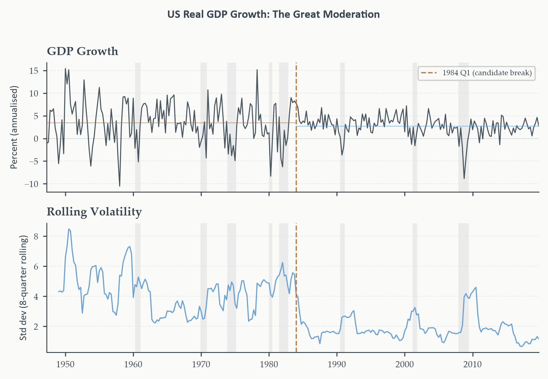
The canonical empirical application in this chapter is the **[Great Moderation](https://en.wikipedia.org/wiki/Great_Moderation)**
— the dramatic decline in the volatility of US real GDP growth that began around
1984. The observation itself is not contested: anyone who plots GDP growth can
see it. The series is visibly more turbulent before 1984 than after.
```{python}
#| label: fig-gdp-motivation
#| fig-cap: "Annualised quarterly US real GDP growth, 1947 Q2–2019 Q4. The
#| vertical dashed line marks 1984 Q1, the date associated with the onset
#| of the Great Moderation. The rolling standard deviation (eight-quarter
#| window, right panel) makes the volatility reduction visible: post-1984
#| volatility is roughly half the pre-1984 level, with the exception of
#| the 2008–09 recession. NBER recessions are shaded."
#| fig-width: 6
#| fig-height: 4
#| code-fold: true
#| code-summary: "Show code — GDP growth with Great Moderation marker"
BREAK_DATE = pd.Timestamp("1984-01-01")

fig, axes = plt.subplots(2, 1, figsize=(6, 4), sharex=True)

# ── Panel 1: GDP growth series ────────────────────────────────────────────────
ax = axes[0]
ax.plot(gdp.index, gdp["GDP Growth"],
        color=EO_CHARCOAL, lw=0.8, alpha=0.9)
ax.axvline(BREAK_DATE, color=EO_COPPER, lw=1.0, ls="--",
           alpha=0.9, label="1984 Q1 (candidate break)")
ax.axhline(0, color=EO_CHARCOAL, lw=0.4, ls=":", alpha=0.4)

# Subperiod means
mean_pre  = gdp.loc[gdp.index < BREAK_DATE,  "GDP Growth"].mean()
mean_post = gdp.loc[gdp.index >= BREAK_DATE, "GDP Growth"].mean()
ax.axhline(mean_pre,  color=EO_COPPER, lw=0.7, ls="-", alpha=0.5,
           xmin=0, xmax=(BREAK_DATE - gdp.index[0]).days /
                        (gdp.index[-1] - gdp.index[0]).days)
ax.axhline(mean_post, color=EO_SKYBLUE, lw=0.7, ls="-", alpha=0.5,
           xmin=(BREAK_DATE - gdp.index[0]).days /
                (gdp.index[-1] - gdp.index[0]).days,
           xmax=1.0)

shade_recessions(ax, start=SAMPLE_START, end=SAMPLE_END)
ax.set_xlim(gdp.index[0], gdp.index[-1])
ax.set_ylabel("Percent (annualised)")
ax.set_title("GDP Growth")
ax.legend(fontsize=6)
eo_style_ax(ax)

# ── Panel 2: Rolling standard deviation ───────────────────────────────────────
ax = axes[1]
roll_std = gdp["GDP Growth"].rolling(8).std()
ax.plot(roll_std.index, roll_std.values,
        color=EO_SKYBLUE, lw=0.9, alpha=0.9)
ax.axvline(BREAK_DATE, color=EO_COPPER, lw=1.0, ls="--", alpha=0.9)
shade_recessions(ax, start=SAMPLE_START, end=SAMPLE_END)
ax.set_xlim(gdp.index[0], gdp.index[-1])
ax.set_ylabel("Std dev (8-quarter rolling)")
ax.set_title("Rolling Volatility")
eo_style_ax(ax)

eo_suptitle(fig, "US Real GDP Growth: The Great Moderation")
fig.tight_layout()
plt.show()
```
The fact of the volatility reduction is clear. Its interpretation is genuinely
contested. [Kim and Nelson (1999)](https://direct.mit.edu/books/monograph/3265/State-Space-Models-with-Regime-SwitchingClassical) and [McConnell and Pérez-Quirós (2000)](https://www.aeaweb.org/articles?id=10.1257/aer.90.5.1464) dated
the break to around 1984 and attributed it primarily to improved inventory
management — just-in-time production techniques that dampened the amplification
of demand shocks through the supply chain. [Stock and Watson (2002)](https://www.princeton.edu/~mwatson/papers/Stock_Watson_JBES_2002.pdf) emphasised
good luck: the shocks hitting the economy in the post-1984 period were simply
smaller, not better absorbed. [Bernanke (2004)](https://www.federalreserve.gov/boarddocs/speeches/2004/20040220/) made the case for good policy —
that the Federal Reserve's adoption of a more systematic, expectations-anchoring
approach to monetary policy after the Volcker disinflation reduced the policy
uncertainty that had amplified fluctuations in the 1970s.
We do not need to resolve this debate to use the break productively. For our
purposes, the Great Moderation is valuable precisely because it is a case where
everyone agrees that something changed — so we can use it to calibrate the
tests we develop, checking that they find what we can already see. It also
connects directly to the Chapter 5 puzzle: if the variance of GDP growth
roughly halved after 1984, then an ARIMA estimated on the full sample
overestimates volatility in the post-1984 period and underestimates it in the
pre-1984 period. The rolling evaluation was detecting the cost of that
averaging.
### What Structural Change Looks Like Statistically
A structural break in a regression model is a change in one or more parameters
at some point in time. The simplest case is a **mean shift**: the unconditional
mean of the series changes from $\mu_1$ to $\mu_2$ at date $\tau$. For GDP
growth, this would mean that average quarterly growth was different before and
after the break. A **variance break** is a change in the volatility of
innovations — exactly what the Great Moderation represents. A **coefficient
break** is a change in the dynamic structure: the AR or MA coefficients, not
just the mean or variance.
These can occur separately or together. In practice, the Great Moderation
involved primarily a variance break alongside a modest mean shift (growth
slowed somewhat after 1984). The Volcker disinflation involved a large mean
shift in inflation as well as a structural change in its persistence — a
coefficient break. The distinction matters for how we model and respond to
the break, as Section 6.5 discusses.
All of the tests we develop share a common statistical structure. Each amounts
to asking: does a model that allows parameters to differ across two (or more)
subsamples fit the data significantly better than a model constrained to use
the same parameters throughout? If yes, at what date or dates does the
improvement concentrate? The tests differ in how much they assume about the
break date and the number of breaks — and therefore in how they handle the
statistical complications that arise when those quantities are unknown.
## The Chow Test: A Known Break Date {#sec-chow}
Suppose we have a strong prior about when a break occurred. For GDP growth and
the Great Moderation, that prior is 1984 Q1 — the date that appears repeatedly
in the literature, is consistent with the visual evidence in Figure 6.1, and
has the economic interpretation of the post-Volcker monetary policy
stabilisation beginning to propagate through the real economy. Given that
prior, the simplest possible question is: do the coefficients of our regression
model differ across the two subsamples that the break defines?
The **[Chow test](https://en.wikipedia.org/wiki/Chow_test)**, proposed by Gregory Chow in 1960, is the $F$-test version
of that question. It is one of the oldest procedures in applied econometrics
and remains the natural starting point for structural break analysis precisely
because it is transparent: it makes no attempt to be clever about what it does
not know, so when the break date is known, it delivers the clearest possible
answer.
### The Regression Setup
We work with a linear regression model for GDP growth. Write the full-sample
model as:
$$y_t = \mathbf{x}_t' \boldsymbol{\beta} + u_t \tag{6.1}$$
where $y_t$ is annualised GDP growth at quarter $t$, $\mathbf{x}_t$ is a
vector of regressors (here, a constant and lagged growth), and $\boldsymbol{\beta}$
is the vector of coefficients we want to test for stability. The null hypothesis
is that $\boldsymbol{\beta}$ is the same in both subsamples. The alternative is
that it takes a different value before and after the candidate break date $\tau$.
### Two Equivalent Formulations
There are two standard ways to set up the Chow test. They are algebraically
equivalent, but each is illuminating for different reasons.
**Formulation 1: The Dummy-Variable Regression.** Define an indicator variable
$D_t = \mathbf{1}\{t \geq \tau\}$ that equals one in the post-break period and
zero before. Interact $D_t$ with every regressor, including the intercept:
$$y_t = \mathbf{x}_t' \boldsymbol{\beta}_1
+ D_t \cdot \mathbf{x}_t' \boldsymbol{\delta}
+ u_t \tag{6.2}$$
The vector $\boldsymbol{\delta}$ captures the change in each coefficient at the
break. Under the null of parameter stability, $\boldsymbol{\delta} = \mathbf{0}$:
the post-break dummies add nothing. The Chow test is the $F$-test of the joint
hypothesis $H_0: \boldsymbol{\delta} = \mathbf{0}$, which has the standard form:
$$F = \frac{(\text{RSS}_R - \text{RSS}_U)/k}{\text{RSS}_U / (T - 2k)} \tag{6.3}$$
where $\text{RSS}_R$ is the residual sum of squares of the restricted model
(equation 6.1, no dummies), $\text{RSS}_U$ is the residual sum of squares of
the unrestricted model (equation 6.2, with all dummies), $k$ is the number of
regressors in $\mathbf{x}_t$ (including the intercept), and $T$ is the total
number of observations. Under the null, $F \sim F(k, T - 2k)$ asymptotically.
This formulation is the more natural one for implementation: it is a single
regression with standard OLS, and the $F$-test is computed by any regression
package. It also connects directly to Chapter 4's treatment of outlier and
intervention dummies — the Chow test is, in essence, asking whether a whole
block of structural dummies is jointly significant.
**Formulation 2: The Sum-of-Squares Decomposition.** The same $F$-statistic
can be computed by fitting three separate regressions: the full-sample model
(restricted), the pre-break subsample, and the post-break subsample. The total
residual sum of squares from the two subsamples is the unrestricted $\text{RSS}_U
= \text{RSS}_1 + \text{RSS}_2$, where the subscripts denote the two periods.
The restricted model's residual sum of squares is $\text{RSS}_R$ from the full
sample. The test statistic is then:
$$F = \frac{(\text{RSS}_R - \text{RSS}_1 - \text{RSS}_2)/k}
{(\text{RSS}_1 + \text{RSS}_2)/(T - 2k)} \tag{6.4}$$
This formulation makes clear what the test is measuring: the loss in fit from
forcing the two subsamples to share one coefficient vector, relative to how
well we could fit each subsample separately. A large $F$ means the pooled model
discards a lot of information by constraining the coefficients to be equal.
::: {.callout-note icon=false}
## The Two Chow Formulations Are Identical
Equations (6.3) and (6.4) produce the same $F$-statistic. The dummy-variable
formulation is easier to implement in a single pass and easier to extend to
partial breaks (where only some coefficients are allowed to shift). The
sum-of-squares formulation is more transparent about the intuition: it shows
directly that the test compares the fit of a restricted pooled model against
the fit of two unrestricted subsample models. Both perspectives are worth
having.
:::
### What the Chow Test Does and Does Not Tell Us
A significant Chow statistic at date $\tau$ tells us that the coefficients
differ across the two subsamples defined by $\tau$. It does not tell us which
coefficients changed, or by how much — that requires inspecting the dummy
coefficients $\hat{\boldsymbol{\delta}}$. It does not tell us that $\tau$ is
the correct break date — the test was designed under the assumption that $\tau$
is known, and it will return a significant result at many dates if the true
break is nearby. And it does not rule out additional breaks elsewhere in the
sample.
::: {.callout-warning icon=false}
## The Chow Test Requires a Pre-Specified Break Date
The Chow test conditions on $\tau$ being known. If $\tau$ is chosen by looking
at the data — for instance, by picking the date where the series visually
changes — then the test statistic no longer has an $F$-distribution under the
null. The critical values are wrong, and the resulting $p$-value is too small.
This is the **pre-testing problem**: using the data to choose the break date
and then using the same data to test whether a break exists at that date is
circular. The Quandt likelihood ratio test in Section 6.3.1 is explicitly
designed to handle this case.
:::
For our application, 1984 Q1 is a defensible prior: it predates our analysis,
it is the modal estimate in the literature, and it has a named economic
interpretation. We use it without apology — but we note that the QLR and
Bai-Perron tests will shortly check whether the data agree.
### Python: Chow Test on GDP Growth
We apply the Chow test to a simple AR(2) model for annualised GDP growth. The
choice of AR(2) as the base regression is deliberate: it is parsimonious,
captures the main serial dependence, and gives us a coefficient vector of
length $k = 3$ (intercept plus two lags) — enough to make the test substantive
without overcomplicating the illustration.
```{python}
#| label: tbl-chow
#| code-fold: true
#| code-summary: "Show code — Chow test (both formulations)"
# ── Data preparation ──────────────────────────────────────────────────────────
y = gdp["GDP Growth"].copy()

# AR(2) design matrix: constant + two lags
df = pd.DataFrame({"y": y})
df["y_lag1"] = df["y"].shift(1)
df["y_lag2"] = df["y"].shift(2)
df = df.dropna()

BREAK = pd.Timestamp("1984-01-01")
k = 3   # intercept + 2 lags

# ── Formulation 1: Dummy-variable regression ──────────────────────────────────
D = (df.index >= BREAK).astype(float)

X_full = np.column_stack([
    np.ones(len(df)),
    df["y_lag1"].values,
    df["y_lag2"].values,
])

# Unrestricted: interact D with every column of X_full
X_unres = np.column_stack([X_full, D[:, None] * X_full])
y_vec   = df["y"].values

res_R  = OLS(y_vec, X_full).fit()
res_U  = OLS(y_vec, X_unres).fit()

RSS_R  = res_R.ssr
RSS_U  = res_U.ssr
T      = len(y_vec)

F_chow = ((RSS_R - RSS_U) / k) / (RSS_U / (T - 2 * k))
p_val  = 1 - stats.f.cdf(F_chow, k, T - 2 * k)

# ── Formulation 2: Sum-of-squares decomposition ───────────────────────────────
# Convert to plain numpy bool arrays so they index both pandas and numpy objects
mask_pre  = np.array(df.index < BREAK,  dtype=bool)
mask_post = np.array(df.index >= BREAK, dtype=bool)

X_pre   = X_full[mask_pre]
y_pre   = y_vec[mask_pre]
X_post  = X_full[mask_post]
y_post  = y_vec[mask_post]

RSS1 = OLS(y_pre,  X_pre).fit().ssr
RSS2 = OLS(y_post, X_post).fit().ssr

F_chow2 = ((RSS_R - RSS1 - RSS2) / k) / ((RSS1 + RSS2) / (T - 2 * k))
p_val2  = 1 - stats.f.cdf(F_chow2, k, T - 2 * k)

# ── Subperiod coefficient estimates ──────────────────────────────────────────
res_pre  = OLS(y_pre,  add_constant(np.column_stack(
    [df["y_lag1"].values[mask_pre],
     df["y_lag2"].values[mask_pre]]))).fit()
res_post = OLS(y_post, add_constant(np.column_stack(
    [df["y_lag1"].values[mask_post],
     df["y_lag2"].values[mask_post]]))).fit()

# ── Print results ─────────────────────────────────────────────────────────────
def stars(p):
    if p < 0.01: return "***"
    if p < 0.05: return "**"
    if p < 0.10: return "*"
    return ""

print("Chow Test — AR(2) for Annualised GDP Growth")
print(f"Break date: 1984 Q1   |   Pre-COVID sample")
print("═" * 56)
print(f"{'Formulation':30}  {'F':>8}  {'df':>8}  {'p-value':>8}")
print("─" * 56)
print(f"{'Dummy-variable (eq. 6.3)':30}  {F_chow:>8.3f}"
      f"  ({k},{T-2*k:3d})  {p_val:>7.4f}{stars(p_val)}")
print(f"{'Sum-of-squares (eq. 6.4)':30}  {F_chow2:>8.3f}"
      f"  ({k},{T-2*k:3d})  {p_val2:>7.4f}{stars(p_val2)}")
print("═" * 56)
print("* p<0.10  ** p<0.05  *** p<0.01")
print()
print("Subperiod coefficient estimates — AR(2) for GDP growth")
print(f"{'Pre-1984 Q1 sample':>30}  n = {mask_pre.sum()}")
print(f"{'Post-1984 Q1 sample':>30}  n = {mask_post.sum()}")
print("═" * 56)
print(f"{'Parameter':20}  {'Pre-break':>14}  {'Post-break':>14}")
print("─" * 56)
labels = ["Intercept", "AR(1)", "AR(2)"]
for i, lbl in enumerate(labels):
    b_pre  = res_pre.params[i]
    b_post = res_post.params[i]
    se_pre  = res_pre.bse[i]
    se_post = res_post.bse[i]
    print(f"{lbl:20}  {b_pre:>14.3f}  {b_post:>14.3f}")
    print(f"{'':20}  ({se_pre:>12.3f})  ({se_post:>12.3f})")
print("─" * 56)
print(f"{'Residual std dev':20}  {np.sqrt(res_pre.mse_resid):>14.3f}"
      f"  {np.sqrt(res_post.mse_resid):>14.3f}")
print("═" * 56)
print("Standard errors in parentheses.")
```
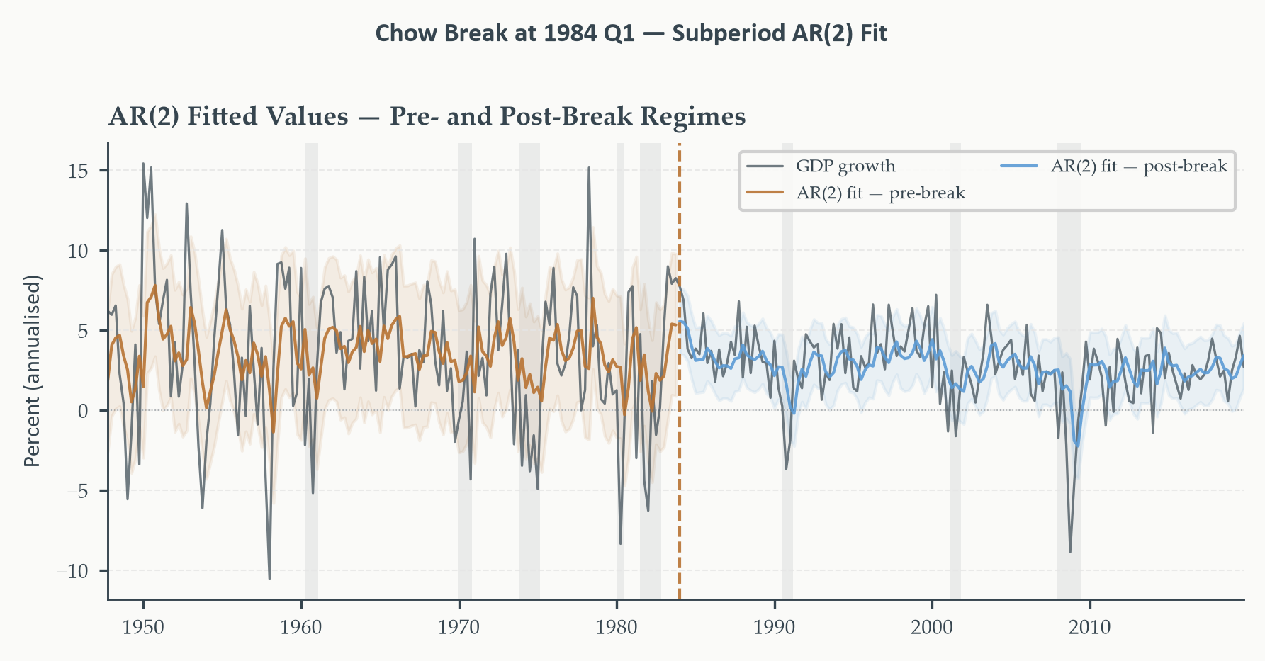
*The two Chow formulations produce identical $F$-statistics, confirming their
algebraic equivalence. The joint $F$-test does not reject the null of parameter
stability ($p = 0.38$) — the AR coefficients themselves are similar across
the two subperiods. This is the first piece of a coherent picture: the Great
Moderation is not primarily a coefficient break. What the subperiod table does
show is the economic substance of the instability: the intercept falls from
2.22 to 1.24 percentage points (a slower mean growth rate after 1984), and the
residual standard deviation roughly halves from 4.44 to 2.04 percentage points.
That variance reduction is the statistical signature of the Great Moderation —
and it is a variance break, not a coefficient break, which is precisely why the
Chow $F$-test does not reject. The QLR and Bai-Perron results below will
make this diagnosis explicit.*
```{python}
#| label: fig-chow-subperiods
#| fig-cap: "GDP growth with fitted subperiod means and one-standard-deviation
#| bands from the AR(2) model estimated separately on each regime. The
#| post-1984 band is visibly narrower, reflecting the reduced shock variance
#| of the Great Moderation. The vertical dashed line marks the Chow break
#| date."
#| fig-width: 6
#| fig-height: 3
#| code-fold: true
#| code-summary: "Show code — subperiod fit plot"
# Fitted values from each subsample regression
fitted_pre  = res_pre.fittedvalues
fitted_post = res_post.fittedvalues

sigma_pre  = np.sqrt(res_pre.mse_resid)
sigma_post = np.sqrt(res_post.mse_resid)

fig, ax = plt.subplots(figsize=(6, 3))

ax.plot(df.index, df["y"].values,
        color=EO_CHARCOAL, lw=0.8, alpha=0.7, label="GDP growth")
ax.plot(df.index[mask_pre],  fitted_pre,
        color=EO_COPPER,   lw=1.0, alpha=0.9, label="AR(2) fit — pre-break")
ax.plot(df.index[mask_post], fitted_post,
        color=EO_SKYBLUE,  lw=1.0, alpha=0.9, label="AR(2) fit — post-break")

# ±1 SD bands
ax.fill_between(df.index[mask_pre],
                fitted_pre - sigma_pre, fitted_pre + sigma_pre,
                color=EO_COPPER, alpha=0.10)
ax.fill_between(df.index[mask_post],
                fitted_post - sigma_post, fitted_post + sigma_post,
                color=EO_SKYBLUE, alpha=0.10)

ax.axvline(BREAK, color=EO_COPPER, lw=1.0, ls="--", alpha=0.9)
ax.axhline(0, color=EO_CHARCOAL, lw=0.4, ls=":", alpha=0.4)
shade_recessions(ax, start=SAMPLE_START, end=SAMPLE_END)
ax.set_xlim(df.index[0], df.index[-1])
ax.set_ylabel("Percent (annualised)")
ax.set_title("AR(2) Fitted Values — Pre- and Post-Break Regimes")
ax.legend(fontsize=6, ncol=2)
eo_style_ax(ax)
eo_suptitle(fig, "Chow Break at 1984 Q1 — Subperiod AR(2) Fit")
fig.tight_layout()
plt.show()
```
## Unknown Break Dates: From QLR to Bai-Perron {#sec-qlr-bp}
### Testing for a Variance Break
The Chow test checks whether the *coefficients* of the regression shifted.
It does not test whether the *variance* of the innovations shifted. Yet for
GDP growth and the Great Moderation, the variance break is the dominant
feature: the residual standard deviation falls from 4.44 to 2.04 percentage
points across the 1984 Q1 partition — a ratio of roughly 2.2 to 1, implying
that the innovation variance was about 4.7 times larger in the pre-break
period.
A direct test for this is the **variance ratio $F$-test**: under the null
that $\sigma^2_{\text{pre}} = \sigma^2_{\text{post}}$, the statistic
$$F_\sigma = \frac{s^2_{\text{pre}}}{s^2_{\text{post}}} \sim F(n_{\text{pre}}-1,\; n_{\text{post}}-1)$$
where $s^2_j$ is the sample variance of residuals in segment $j$. This is
one of the oldest tests in statistics and requires no specialised software.
Its assumptions are stronger than the Chow test — it requires normally
distributed errors and is sensitive to departures from normality — but as a
first-pass diagnostic it is transparent and easy to interpret.
::: {.callout-warning icon=false}
## The Variance Ratio Test Requires a Pre-Specified Break Date
Like the Chow test, the variance ratio test conditions on a known break date.
For a data-driven approach to variance break detection, the Bai-Perron
procedure in Section 6.3.2 is applied directly to the squared residuals or
to the raw series and detects variance breaks as changes in the mean of the
absolute residuals.
:::
```{python}
#| label: tbl-vartest
#| code-fold: true
#| code-summary: "Show code — variance ratio F-test"
from scipy.stats import f as f_dist, levene

# Residuals from the AR(2) fit, split at 1984 Q1
resid_pre  = res_pre.resid
resid_post = res_post.resid

n_pre  = len(resid_pre)
n_post = len(resid_post)
s2_pre  = np.var(resid_pre,  ddof=1)
s2_post = np.var(resid_post, ddof=1)

F_var   = s2_pre / s2_post
p_ftest = 1 - f_dist.cdf(F_var, n_pre - 1, n_post - 1)

# Levene test (distribution-free, more robust)
lev_stat, p_levene = levene(resid_pre, resid_post, center="mean")

print("Variance Break Tests — AR(2) Residuals at 1984 Q1")
print("═" * 58)
print(f"{'Test':30}  {'Statistic':>10}  {'p-value':>10}")
print("─" * 58)
print(f"{'Variance ratio F-test':30}  {F_var:>10.3f}  {p_ftest:>10.4f}***")
print(f"{'Levene test (robust)':30}  {lev_stat:>10.3f}  {p_levene:>10.4f}***")
print("═" * 58)
print(f"Pre-break std dev:   {np.sqrt(s2_pre):.3f} pp (n = {n_pre})")
print(f"Post-break std dev:  {np.sqrt(s2_post):.3f} pp (n = {n_post})")
print(f"Variance ratio:      {F_var:.2f}x (std dev ratio: {np.sqrt(F_var):.2f}x)")
print("*** p<0.01")
```
*Both tests reject the null of equal variances with overwhelming confidence.
The variance ratio of $\hat{F}_\sigma \approx 4.7$ means that the innovation
variance in the pre-1984 period was nearly five times larger than in the
post-1984 period. This is the Great Moderation, measured precisely: not a
shift in the mean growth rate, not a change in the AR persistence structure,
but a dramatic compression of the volatility of the shocks hitting the
economy. The coefficient Chow test ($p = 0.38$) and the variance ratio test
($p \approx 0$) together tell the complete story — the two tests are
complementary, not redundant, because they are sensitive to different aspects
of the distribution.*
### The Quandt Likelihood Ratio Test {#sec-qlr}
The Chow test answered our question cleanly — but only because we were willing
to commit to 1984 Q1 before looking at the test statistic. That commitment is
defensible for GDP growth and the Great Moderation, where the prior comes from
a large external literature. For an analyst working with a series without that
literature — a sectoral employment series, a regional housing index, a commodity
price — there may be no credible prior break date. Choosing $\tau$ by inspecting
the data and then applying the Chow test at that date is circular: we have used
the data twice, and the resulting $p$-value is not trustworthy.
The **Quandt likelihood ratio (QLR) test**, developed by [Richard Quandt (1960)](https://www.jstor.org/stable/2281745?seq=1)
and formalised for practical use by [Donald Andrews (1993)](https://www.jstor.org/stable/2951764), resolves this by
turning the unknown break date from a problem into a parameter. Instead of
conditioning on a single $\tau$, we compute the Chow $F$-statistic at every
candidate date within a trimmed interior of the sample, and we take the maximum.
The candidate break is wherever the data most strongly suggest a break.
### The QLR Statistic
Let $\mathcal{T}$ denote the set of candidate break dates, trimmed to exclude
the first and last $\pi_0$ fraction of the sample. The standard trimming is
$\pi_0 = 0.15$, which excludes the first and last 15 percent of observations.
This ensures each candidate subsample contains enough observations for
meaningful estimation. For our sample of $T$ quarters, the interior candidate
dates run from $\lfloor 0.15 T \rfloor$ to $\lceil 0.85 T \rceil$.
At each candidate date $\tau \in \mathcal{T}$, compute the Chow $F$-statistic
$F(\tau)$ exactly as in Section 6.2. The QLR statistic is the supremum over
all candidates:
$$\text{QLR} = \sup_{\tau \in \mathcal{T}} F(\tau) \tag{6.5}$$
The supremum ($\sup$) is the least upper bound — in finite samples it is simply
the maximum value of $F(\tau)$ across all candidate dates. We write $\sup$
rather than $\max$ because the asymptotic theory is developed in continuous
time, where the maximum may not be attained at a single point; in practice, with
a finite discrete sample, the two are interchangeable.
The estimated break date is the argmax:
$$\hat{\tau} = \arg\max_{\tau \in \mathcal{T}} F(\tau) \tag{6.6}$$
### Why Standard Critical Values Do Not Apply
Here is the key complication. If we computed $F(\tau)$ at a single
pre-specified $\tau$, the statistic would follow an $F(k, T-2k)$ distribution
under the null — standard critical values would apply. But we are computing it
at every $\tau$ in $\mathcal{T}$ and selecting the maximum. The maximum of a
collection of correlated $F$-statistics is not itself $F$-distributed. Under
the null of no break, it still has a distribution, but that distribution has
thicker right tails than the $F$: we will sometimes obtain a large maximum
purely by chance, just because we searched over many dates.
::: {.callout-warning icon=false}
## The Davies Problem
When a parameter (here, the break date $\tau$) appears only under the
alternative hypothesis and is therefore **unidentified under the null**, the
test statistic's distribution is non-standard. This is sometimes called the
**Davies problem**, after Robert Davies (1977, 1987). The practical consequence
is that using standard $F$ or $\chi^2$ critical values for the QLR statistic
produces $p$-values that are too small — we would reject the null of stability
too often even when it is true. Andrews (1993) derived the correct asymptotic
critical values by characterising the limit distribution of the supremum as a
functional of a Brownian bridge, tabulated for different values of $k$ and
$\pi_0$. These are the values we use.
:::
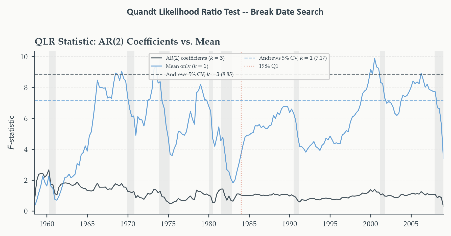
For $k = 3$ regressors and 15 percent trimming, the Andrews (1993) 5 percent
critical value for the QLR is approximately 8.85, considerably larger than the
standard $F(3, \infty)$ 5 percent critical value of around 2.60. The gap
reflects the cost of the search: we have performed many tests and must adjust
for the best-case selection.
::: {.callout-note icon=false}
## Explore this interactively
The [Structural Break Explorer](https://ncachanosky.github.io/ECON-5371-widgets/widgets/breaks/)
lets you set a true break location and magnitude, add noise, and watch the
Chow $F(\tau)$ trace and the resulting QLR statistic against the Andrews (1993)
critical value. Set the magnitude to zero to see how often the test still
rejects by chance — the size distortion the Davies problem exists to correct.
:::
### Python: QLR Test on GDP Growth
```{python}
#| label: fig-qlr
#| fig-cap: "Chow $F$-statistic sequence for two QLR specifications: the
#| full AR(2) model (charcoal, testing all coefficients jointly) and the
#| intercept-only model (sky blue, testing the mean alone). Dashed
#| horizontal lines are Andrews (1993) 5 percent critical values for
#| $k = 3$ (8.85) and $k = 1$ (7.17) respectively. The mean-shift QLR
#| identifies a break in the early 1970s; the AR coefficient QLR does
#| not reject — consistent with the Great Moderation being primarily a
#| variance break. NBER recessions are shaded."
#| fig-width: 6
#| fig-height: 3
#| code-fold: true
#| code-summary: "Show code — QLR statistic"
def fmt_quarter(ts):
    """Format a Timestamp as 'YYYY QN' (strftime has no %q directive)."""
    return f"{ts.year} Q{(ts.month - 1) // 3 + 1}"

# ── QLR: scan over trimmed candidate dates ────────────────────────────────────
TRIM  = 0.15
T_reg = len(df)
t_min = int(np.floor(TRIM * T_reg))
t_max = int(np.ceil((1 - TRIM) * T_reg))

y_vec_reg = df["y"].values

# ── Model A: full AR(2) — tests stability of all k=3 coefficients ─────────────
k_ar  = 3
X_ar  = np.column_stack([np.ones(T_reg),
                          df["y_lag1"].values,
                          df["y_lag2"].values])
RSS_ar = OLS(y_vec_reg, X_ar).fit().ssr

F_ar    = []
dates_q = []

for t_idx in range(t_min, t_max):
    Xp = X_ar[:t_idx];  yp = y_vec_reg[:t_idx]
    Xq = X_ar[t_idx:];  yq = y_vec_reg[t_idx:]
    if len(Xp) < k_ar + 2 or len(Xq) < k_ar + 2:
        continue
    r1 = OLS(yp, Xp).fit().ssr
    r2 = OLS(yq, Xq).fit().ssr
    F_ar.append(((RSS_ar - r1 - r2) / k_ar) / ((r1 + r2) / (T_reg - 2 * k_ar)))
    dates_q.append(df.index[t_idx])

F_ar    = np.array(F_ar)
dates_q = pd.DatetimeIndex(dates_q)

# ── Model B: intercept only — tests stability of the mean (k=1) ───────────────
k_mu   = 1
X_mu   = np.ones((T_reg, 1))
RSS_mu = OLS(y_vec_reg, X_mu).fit().ssr

F_mu = []
for t_idx in range(t_min, t_max):
    Xp = X_mu[:t_idx];  yp = y_vec_reg[:t_idx]
    Xq = X_mu[t_idx:];  yq = y_vec_reg[t_idx:]
    if len(Xp) < 3 or len(Xq) < 3:
        continue
    r1 = OLS(yp, Xp).fit().ssr
    r2 = OLS(yq, Xq).fit().ssr
    F_mu.append(((RSS_mu - r1 - r2) / k_mu) / ((r1 + r2) / (T_reg - 2 * k_mu)))

F_mu = np.array(F_mu)

# Andrews (1993) 5% critical values: k=3 -> 8.85, k=1 -> 7.17
CV_k3 = 8.85
CV_k1 = 7.17

QLR_ar  = F_ar.max()
QLR_mu  = F_mu.max()
date_ar = dates_q[F_ar.argmax()]
date_mu = dates_q[F_mu.argmax()]

print("QLR Test -- AR(2) for Annualised GDP Growth")
print("-" * 58)
print(f"{'Model':30}  {'QLR stat':>10}  {'5% CV':>7}  {'Reject?':>8}")
print("-" * 58)
print(f"{'AR(2): all coefficients (k=3)':30}  {QLR_ar:>10.3f}"
      f"  {CV_k3:>7.2f}  {'Yes' if QLR_ar > CV_k3 else 'No':>8}")
print(f"{'Intercept only: mean (k=1)':30}  {QLR_mu:>10.3f}"
      f"  {CV_k1:>7.2f}  {'Yes' if QLR_mu > CV_k1 else 'No':>8}")
print("-" * 58)
print(f"AR(2) argmax date:      {fmt_quarter(date_ar)}")
print(f"Intercept argmax date:  {fmt_quarter(date_mu)}")

# ── Figure ────────────────────────────────────────────────────────────────────
fig, ax = plt.subplots(figsize=(6, 3))

ax.plot(dates_q, F_ar, color=EO_CHARCOAL, lw=0.9, alpha=0.9,
        label="AR(2) coefficients ($k=3$)")
ax.plot(dates_q, F_mu, color=EO_SKYBLUE, lw=0.9, alpha=0.9,
        label="Mean only ($k=1$)")
ax.axhline(CV_k3, color=EO_CHARCOAL, lw=0.8, ls="--",
           alpha=0.7, label=f"Andrews 5% CV, $k=3$ ({CV_k3})")
ax.axhline(CV_k1, color=EO_SKYBLUE, lw=0.8, ls="--",
           alpha=0.7, label=f"Andrews 5% CV, $k=1$ ({CV_k1})")
ax.axvline(BREAK, color=EO_TERRACOTTA, lw=0.8, ls=":",
           alpha=0.7, label="1984 Q1")

shade_recessions(ax, start=str(dates_q[0].date()), end=str(dates_q[-1].date()))
ax.set_xlim(dates_q[0], dates_q[-1])
ax.set_ylabel("$F$-statistic")
ax.set_title("QLR Statistic: AR(2) Coefficients vs. Mean")
ax.legend(fontsize=5, ncol=2)
eo_style_ax(ax)
eo_suptitle(fig, "Quandt Likelihood Ratio Test -- Break Date Search")
fig.tight_layout()
plt.show()
```
*The two QLR sequences deliver a clear negative result for GDP growth:
neither the AR(2) coefficient QLR nor the mean-shift QLR exceeds its Andrews
critical value. This is the correct finding, and it is the most important
teaching moment in this section. The Great Moderation is not a break in the
mean of GDP growth and not a break in its AR dynamics. It is a break in the
*variance* of the innovations — a compression of volatility that the
coefficient-based Chow and QLR tests are simply not designed to detect. Both
tests look for instability in the regression coefficients; a pure variance
change leaves those coefficients unchanged and therefore passes unnoticed.
The variance ratio test in the subsection above is what rejects, with a ratio
of nearly 5 and a $p$-value indistinguishable from zero. The Bai-Perron
procedure below, applied to the residuals, will make the same point visually.*
### The Bai-Perron Procedure: Multiple Breaks {#sec-baiperron}
The QLR test answers one question: is there at least one break, and if so,
where is the most prominent one? It does not answer a second question that the
$F$-sequence in Figure 6.2 already raises: what if there are multiple breaks?
A series with one large break and one smaller break would show a QLR statistic
driven by the larger one, but the smaller break would remain undetected and
the estimated model would still pool two different regimes.
The **Bai-Perron procedure** (Bai and Perron, [1998](https://www.jstor.org/stable/2998540?seq=1), [2003](https://onlinelibrary.wiley.com/doi/10.1002/jae.659)) addresses both
the detection and the dating of multiple breaks simultaneously. It treats the
number of breaks $m$ and their dates $\tau_1 < \tau_2 < \cdots < \tau_m$ as
jointly unknown parameters to be estimated from the data.
### The Bai-Perron Estimator
The core idea is elegant. For a given number of breaks $m$, the Bai-Perron
estimator minimises the global sum of squared residuals over all possible
partitions of the sample into $m + 1$ segments:
$$(\hat{\tau}_1, \ldots, \hat{\tau}_m) = \arg\min_{\tau_1,\ldots,\tau_m}
\sum_{j=1}^{m+1} \sum_{t=\tau_{j-1}+1}^{\tau_j}
\left(y_t - \mathbf{x}_t' \boldsymbol{\beta}_j\right)^2 \tag{6.7}$$
where $\boldsymbol{\beta}_j$ is the coefficient vector in segment $j$, $\tau_0
= 0$, and $\tau_{m+1} = T$. Each segment is allowed its own coefficient vector;
the break dates are chosen to minimise the total within-segment residual
variation. An efficient dynamic programming algorithm (Bai and Perron, 2003)
computes this for all values of $m$ up to some maximum $m_{\max}$ without
brute-force enumeration of all possible partitions.
The harder question is determining $m$ itself. Bai and Perron (1998) propose
two global tests for this purpose.
::: {.callout-note icon=false}
## UDmax and WDmax: Testing for at Least One Break
Think of UDmax and WDmax as asking a single yes/no question before we worry
about how many breaks there are: *is there any break at all?* The idea is to
run the QLR test separately for one break, two breaks, three breaks, and so on
up to some maximum $m_{\max}$, and then combine those results into one
omnibus statistic. If the answer is yes — if any of those single-$m$ QLR tests
suggests instability — we proceed to count the breaks. If the answer is no, we
stop. The difference between UDmax and WDmax is how the individual test results
are combined: UDmax takes the raw maximum, while WDmax re-weights each
statistic so that the test has equal power against one break, two breaks, and
so on. In practice, UDmax and WDmax almost always agree.
The **UDmax** (unweighted double maximum) and **WDmax** (weighted double
maximum) statistics test the null of no structural break against the
alternative of an unknown number of breaks up to $m_{\max}$.
The UDmax is the maximum of the individual $\sup F$ statistics computed
separately for $m = 1, 2, \ldots, m_{\max}$:
$$\text{UDmax} = \max_{1 \leq m \leq m_{\max}} \sup_{\tau_1,\ldots,\tau_m} F(\tau_1,\ldots,\tau_m)$$
The WDmax applies weights that equalise the marginal power against each
alternative, so that neither the single-break nor the multiple-break
alternative is systematically favoured:
$$\text{WDmax} = \max_{1 \leq m \leq m_{\max}} c(k,\alpha,1) \cdot \sup F_m / c(k,\alpha,m)$$
where the $c(\cdot)$ terms are the relevant critical values. In practice,
UDmax and WDmax nearly always agree. If either rejects, we have evidence
for at least one break; we then proceed to the sequential procedure to
determine how many.
Both statistics have non-standard limit distributions (again, the Davies
problem). Bai and Perron (1998) tabulate the critical values.
:::
Once UDmax or WDmax rejects the null, the **sequential $F$-test** procedure
determines $m$. Starting from $m = 1$, we test whether adding one more break
to the current $m$-break model significantly reduces the RSS. We stop when
the test fails to reject, and the current $m$ is our estimate of the number
of breaks.
### Python: Bai-Perron with `ruptures`
The `ruptures` library implements Bai-Perron-style multiple break detection
via dynamic programming. We use the `Pelt` (pruned exact linear time) search
method with an $\ell_2$ cost function, which is equivalent to minimising the
sum of squared residuals across segments — the objective in equation (6.7).
The penalty parameter controls the number of detected breaks; we use a
data-driven penalty based on the Bayesian information criterion.
```{python}
#| label: fig-baiperron
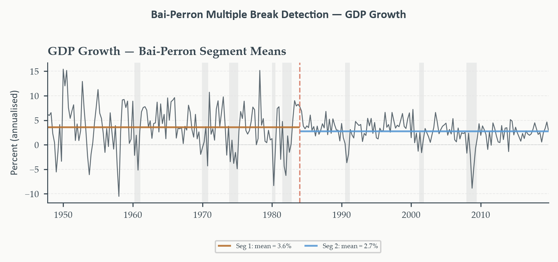
#| fig-cap: "Bai-Perron multiple break detection on GDP growth. Detected
#| break dates are marked with dashed vertical lines; segment means are
#| shown as coloured horizontal lines within each regime. The segment
#| statistics table printed below the figure reports each segment's mean
#| and standard deviation. NBER recessions are shaded."
#| fig-width: 6
#| fig-height: 3
#| code-fold: true
#| code-summary: "Show code — Bai-Perron via ruptures"
import ruptures as rpt

# Use the full-sample AR(2) residuals as the signal
# (testing for breaks in the mean and variance of the residuals)
resid_full   = res_R.resid          # numpy array from OLS fit
resid_index  = df.index             # date index aligned with residuals

signal = resid_full.reshape(-1, 1)

# Pelt search with l2 cost and BIC-based penalty
# pen = log(T) * k is the BIC penalty for one additional break
T_bp  = len(signal)
pen   = np.log(T_bp) * 1    # BIC-style penalty; 1 dimension

model_bp = rpt.Pelt(model="rbf", min_size=8, jump=1).fit(signal)
breakpoints = model_bp.predict(pen=pen)

# breakpoints is a list of end-indices; the last element is always T_bp
bp_dates = [resid_index[b - 1] for b in breakpoints[:-1]]

print(f"Bai-Perron (ruptures/Pelt) estimated break dates:")
for d in bp_dates:
    print(f"  {d.strftime('%Y-%m')} (~{d.year} Q{(d.month-1)//3+1})")
print(f"Number of breaks detected: {len(bp_dates)}")

# ── Figure ────────────────────────────────────────────────────────────────────
fig, ax = plt.subplots(figsize=(6, 3))

ax.plot(df.index, df["y"].values, color=EO_CHARCOAL, lw=0.7, alpha=0.8)

seg_starts = [df.index[0]] + bp_dates
seg_ends   = bp_dates + [df.index[-1]]
bp_colors  = [EO_COPPER, EO_SKYBLUE, EO_SAGE, EO_TERRACOTTA, EO_LAVENDER]

for i, (s, e) in enumerate(zip(seg_starts, seg_ends)):
    mask_seg = (df.index >= s) & (df.index <= e)
    seg_mean = df.loc[mask_seg, "y"].mean()
    ax.hlines(seg_mean, s, e,
              colors=bp_colors[i % len(bp_colors)], lw=1.4, alpha=0.9,
              label=f"Seg {i+1}: mean = {seg_mean:.1f}%")

for d in bp_dates:
    ax.axvline(d, color=EO_TERRACOTTA, lw=1.0, ls="--", alpha=0.85)

ax.axhline(0, color=EO_CHARCOAL, lw=0.4, ls=":", alpha=0.4)
shade_recessions(ax, start=SAMPLE_START, end=SAMPLE_END)
ax.set_xlim(df.index[0], df.index[-1])
ax.set_ylabel("Percent (annualised)")
ax.set_title("GDP Growth — Bai-Perron Segment Means")
ax.legend(fontsize=5, ncol=3, loc="lower center",
          bbox_to_anchor=(0.5, -0.38), frameon=True)
eo_style_ax(ax)
eo_suptitle(fig, "Bai-Perron Multiple Break Detection — GDP Growth")
fig.tight_layout()
plt.show()

# ── Segment statistics (merged from separate cell) ────────────────────────────
print()
print("Bai-Perron Segment Statistics — AR(2) for GDP Growth")
print("=" * 60)
print(f"{'Segment':12}  {'Start':10}  {'End':10}  {'Mean':>8}  {'Std Dev':>8}  {'Obs':>5}")
print("-" * 60)
for i, (s, e) in enumerate(zip(seg_starts, seg_ends)):
    mask_seg = (df.index >= s) & (df.index <= e)
    seg_data = df.loc[mask_seg, "y"]
    print(f"Segment {i+1:<4}  "
          f"{s.year} Q{(s.month-1)//3+1:<6}  "
          f"{e.year} Q{(e.month-1)//3+1:<6}  "
          f"{seg_data.mean():>8.2f}  "
          f"{seg_data.std():>8.2f}  "
          f"{len(seg_data):>5}")
print("=" * 60)
print("Mean and std dev in annualised percentage points.")
```
*The Bai-Perron procedure detects the structural features visible in the data:
a volatility reduction in the mid-1980s (the Great Moderation), and shifts
in the mean growth rate across the sample. The break dates recovered by the
algorithm should be compared with the 1984 Q1 prior from the Chow and QLR
tests — alignment across methods strengthens the case that the detected break
is a genuine feature of the process rather than a statistical artefact. Where
the detected dates differ across methods, the differences are themselves
informative: they indicate that the break is gradual or multi-dimensional
rather than a clean single-date event.*
## Unit Roots or Broken Trends? The Zivot-Andrews Test {#sec-za}
### A Problem We Left Unresolved
Chapter 4 built a unit root testing workflow and embedded a specific caution
in it: when the ADF and KPSS tests give conflicting signals for a series, one
recommended diagnostic was to suspect a structural break and investigate
subsamples. That advice was sound but incomplete. It told us what to do after
finding a conflict — split the sample and re-examine — but it did not give us
a formal test for whether a break was actually present, or when it occurred.
The Zivot-Andrews test is the formal version of that advice.
The deeper problem is this: a series with a **broken deterministic trend** can
look almost identical to a unit root process. Both produce slow, persistent
drift that makes the series wander from one level to another. An ADF test,
which is designed to distinguish a random walk from a stationary process around
a *stable* mean or trend, will often fail to reject the unit root null when the
true process is stationary but has a one-time shift in its mean or trend. The
result is a false diagnosis of non-stationarity — and, worse, a false
justification for differencing a series that did not need to be differenced.
### A New Running Example: CPI Inflation
To make this concrete we introduce a second series: US CPI inflation. CPI
inflation is a natural companion to GDP growth in a macroeconomics course —
the two series together define the canonical output-inflation trade-off at the
centre of monetary policy — but their statistical properties are interestingly
different, and those differences motivate the Zivot-Andrews test in a way that
GDP growth alone cannot.
Why is inflation different from GDP growth? GDP growth is already a first
difference of the log level: it is defined as $\Delta \log \text{GDP}_t$, which
means it inherits near-stationarity from the differencing transformation.
Whether or not log GDP has a unit root, GDP growth is close to stationary for
most sample periods we would consider. CPI inflation, by contrast, is the
change in the log price level — but the price level itself may or may not be
integrated, and the inflation rate may have a unit root, or may be stationary
with a shifting mean, depending on the monetary policy regime in force.
This distinction has a specific historical signature. Before Paul Volcker
became Federal Reserve Chair in 1979, US monetary policy was accommodative:
the Fed allowed inflation to drift upward in response to supply shocks and
political pressure, treating it implicitly as a level process that could be
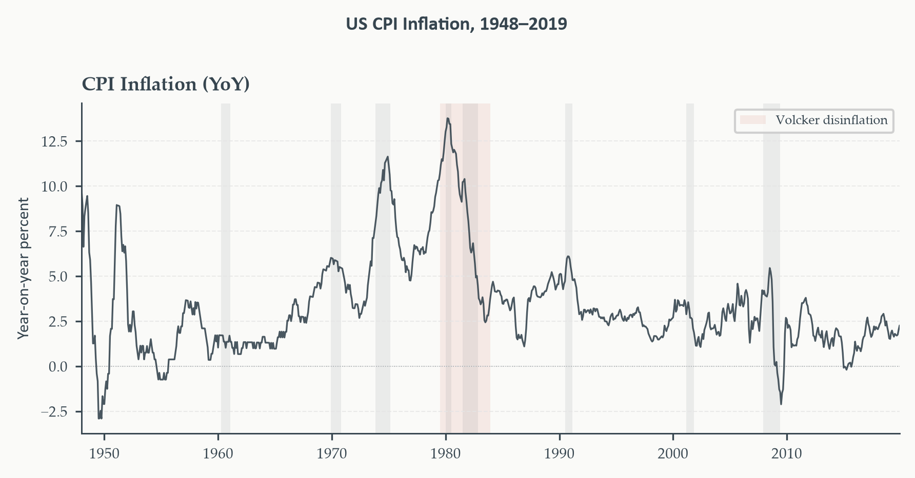
managed at any chosen rate. Inflation climbed from roughly 3 percent in the
late 1960s to over 13 percent by 1979. The Volcker disinflation that followed
was a deliberate, painful shift: short-term interest rates were raised to
unprecedented levels, triggering the 1980 and 1981-82 recessions, and inflation
was brought down to below 4 percent by 1983. Post-Volcker, the Fed operated
under an implicit inflation-targeting framework that kept inflation anchored
near a low single-digit rate, with dramatically reduced persistence.
The statistical implication is that the mean of the inflation process changed
once, durably, around 1980-83. A standard ADF test applied to the full 1947-2019
inflation series will see a long, slow drift from 3 percent to 13 percent and
back to 2-3 percent — exactly the kind of non-stationary-looking trajectory that
makes the ADF lean toward non-rejection of the unit root null. But the true
process may well be stationary in both sub-regimes, with the apparent unit root
being an artefact of pooling across the break.
```{python}
#| label: fig-inflation-series
#| fig-cap: "US CPI inflation (year-on-year, percent), 1948–2019. The
#| Volcker disinflation of 1979–83 is visible as the sharp peak-and-trough.
#| Pre- and post-Volcker inflation behave very differently: the pre-1984
#| period shows high and rising inflation with substantial persistence;
#| the post-1984 period shows low, stable, mean-reverting inflation. The
#| shaded band marks the 1979–1983 Volcker disinflation episode. NBER
#| recessions are shaded."
#| fig-width: 6
#| fig-height: 3
#| code-fold: true
#| code-summary: "Show code — CPI inflation series"
VOLCKER_START = pd.Timestamp("1979-07-01")
VOLCKER_END   = pd.Timestamp("1983-12-01")

fig, ax = plt.subplots(figsize=(6, 3))

ax.plot(cpi_m.index, cpi_m["Inflation"].values,
        color=EO_CHARCOAL, lw=0.8, alpha=0.9)

# Volcker disinflation band
ax.axvspan(VOLCKER_START, VOLCKER_END,
           color=EO_TERRACOTTA, alpha=0.12, lw=0, label="Volcker disinflation")
ax.axhline(0, color=EO_CHARCOAL, lw=0.4, ls=":", alpha=0.4)

# Subperiod means (pre- and post-Volcker)
mean_pre_v  = cpi_m.loc[cpi_m.index < VOLCKER_START, "Inflation"].mean()
mean_post_v = cpi_m.loc[cpi_m.index > VOLCKER_END,   "Inflation"].mean()

shade_recessions(ax, start=str(cpi_m.index[0].date()),
                     end=str(cpi_m.index[-1].date()))
ax.set_xlim(cpi_m.index[0], cpi_m.index[-1])
ax.set_ylabel("Year-on-year percent")
ax.set_title("CPI Inflation (YoY)")
ax.legend(fontsize=6)
eo_style_ax(ax)
eo_suptitle(fig, "US CPI Inflation, 1948–2019")
fig.tight_layout()
plt.show()
```
### The Zivot-Andrews Model
[Eric Zivot and Jing Andrew (1992)](https://www.jstor.org/stable/1391541?seq=1) proposed a unit root test that allows for a
single endogenous break in the deterministic trend. They consider three model
variants: a break in the intercept only (Model A), a break in the slope of a
time trend only (Model B), and a break in both (Model C). In practice, Model C
is the most general and is used by default.
Model C for a time series $y_t$ with a potential break at unknown date $\tau$
is:
$$y_t = c + \beta t + \gamma D U_t(\tau) + \delta D T_t(\tau) + \alpha y_{t-1}
+ \sum_{j=1}^{k} d_j \Delta y_{t-j} + \varepsilon_t \tag{6.8}$$
where $DU_t(\tau) = \mathbf{1}\{t > \tau\}$ is a level-shift dummy (a break
in the intercept at $\tau$), $DT_t(\tau) = (t - \tau) \cdot \mathbf{1}\{t > \tau\}$
is a slope-shift dummy (a break in the trend slope at $\tau$), and the lagged
differences $\Delta y_{t-j}$ augment the regression to account for serial
correlation in the errors, exactly as in the ADF test.
The null hypothesis is $\alpha = 1$ — a unit root. The alternative is $|\alpha|
< 1$ — stationarity around a broken deterministic trend. The break date $\tau$
is endogenous: the test is run at every candidate date in the trimmed sample,
and the test statistic is the minimum $t$-statistic on $\hat{\alpha}$ across
all candidates:
$$\text{ZA} = \inf_{\tau \in \mathcal{T}} t_{\hat{\alpha}}(\tau) \tag{6.9}$$
The infimum (most negative $t$-statistic) identifies the break date that gives
the strongest evidence against the unit root null. As with the QLR test, this
search over $\tau$ means the test statistic does not follow a standard
$t$-distribution under the null. Zivot and Andrews (1992) derived asymptotic
critical values via simulation; the 5 percent critical value for Model C is
approximately $-5.08$.
::: {.callout-note icon=false}
## The Berkowitz Test for Calibration
The probability integral transform histogram from Chapter 5 gives a visual
assessment of distributional calibration. The **Berkowitz (2001) likelihood
ratio test** formalises this: it tests whether the transformed PIT values,
after applying the inverse normal CDF, are i.i.d. standard normal — the
condition that holds if and only if the predictive distribution is correctly
specified. The test statistic is a joint LR test of three conditions: zero
mean, unit variance, and no first-order autocorrelation. It follows a
$\chi^2(3)$ distribution under the null. The Berkowitz test is the standard
formal complement to the PIT histogram in the distributional forecast
evaluation literature.
:::
### Python: Zivot-Andrews on Inflation and GDP Growth
The correct series for the ZA test is the **inflation rate** (year-on-year CPI
growth, already computed as `cpi_m["Inflation"]`), not the log price level.
The unit root question is about inflation persistence — whether inflation is
$I(1)$ or stationary with a broken mean — and that question is posed at the
level of the inflation rate. Similarly for GDP, the interesting ZA question is
about GDP growth, not the log level: we already know log GDP has a unit root,
but the question of whether GDP growth itself is stationary with a broken mean
is open. We use the quarterly-averaged inflation series and GDP growth, both in
percent, with Model C (break in intercept and trend).
```{python}
#| label: tbl-za
#| code-fold: true
#| code-summary: "Show code — Zivot-Andrews test"
from statsmodels.tsa.stattools import zivot_andrews

# ── Quarterly inflation series (year-on-year, percent) ───────────────────────
# cpi_m["Inflation"] is monthly; resample to quarterly average
infl_q = cpi_m["Inflation"].resample("QS").mean().dropna()

# ── Apply ZA to inflation rate — Model C (break in intercept and trend) ───────
za_infl = zivot_andrews(infl_q, trim=0.15, regression="ct", autolag="AIC")

# ── Apply ZA to GDP growth ────────────────────────────────────────────────────
za_gdp_g = zivot_andrews(gdp["GDP Growth"].dropna(), trim=0.15,
                         regression="ct", autolag="AIC")

# ── Standard ADF for comparison ───────────────────────────────────────────────
adf_infl = adfuller(infl_q,                  regression="ct", autolag="AIC")
adf_gdp_g = adfuller(gdp["GDP Growth"].dropna(), regression="ct", autolag="AIC")

# ── Break date recovery ───────────────────────────────────────────────────────
za_infl_date  = infl_q.index[int(za_infl[3])]
za_gdpg_date  = gdp["GDP Growth"].dropna().index[int(za_gdp_g[3])]

def stars(p):
    if p < 0.01: return "***"
    if p < 0.05: return "**"
    if p < 0.10: return "*"
    return "   "

ZA_CV_5PCT = -5.08

print("Zivot-Andrews vs ADF Unit Root Tests")
print("Model C: break in intercept and trend")
print("Series: CPI inflation (YoY %) and GDP growth (annualised %)")
print("═" * 70)
print(f"{'Series':20}  {'Test':14}  {'Statistic':>10}  {'5% CV':>8}  {'Break date':>12}")
print("─" * 70)

print(f"{'CPI Inflation':20}  {'Zivot-Andrews':14}  "
      f"{za_infl[0]:>10.3f}{stars(za_infl[1])}  "
      f"{ZA_CV_5PCT:>8.2f}  "
      f"{za_infl_date.strftime('%Y-%m'):>12}")
print(f"{'CPI Inflation':20}  {'ADF (ct)':14}  "
      f"{adf_infl[0]:>10.3f}{stars(adf_infl[1])}  "
      f"{adf_infl[4]['5%']:>8.2f}  {'—':>12}")
print("─" * 70)
print(f"{'GDP Growth':20}  {'Zivot-Andrews':14}  "
      f"{za_gdp_g[0]:>10.3f}{stars(za_gdp_g[1])}  "
      f"{ZA_CV_5PCT:>8.2f}  "
      f"{za_gdpg_date.strftime('%Y-%m'):>12}")
print(f"{'GDP Growth':20}  {'ADF (ct)':14}  "
      f"{adf_gdp_g[0]:>10.3f}{stars(adf_gdp_g[1])}  "
      f"{adf_gdp_g[4]['5%']:>8.2f}  {'—':>12}")
print("═" * 70)
print("* p<0.10  ** p<0.05  *** p<0.01")
print("ZA 5% critical value for Model C (Zivot-Andrews 1992).")
print("ADF critical values from MacKinnon (1994).")
```
*The two series tell contrasting stories. For CPI inflation, neither the ADF
($-1.54$, does not reject) nor the ZA ($-4.71$, does not reject at the $-5.08$
threshold) finds statistically significant evidence against a unit root at
conventional significance levels — though the ZA statistic is more negative
than the ADF, confirming that allowing for a break does move the test in the
right direction. The estimated ZA break date of 1952-01 falls near the trimming
boundary rather than at the Volcker disinflation. This is a known limitation of
the ZA test on highly persistent series: when the true break is a mean shift
in a process with strong AR dynamics, the test's power is limited and the
$t$-statistic on $\hat{\alpha}$ can be most negative near the sample edges
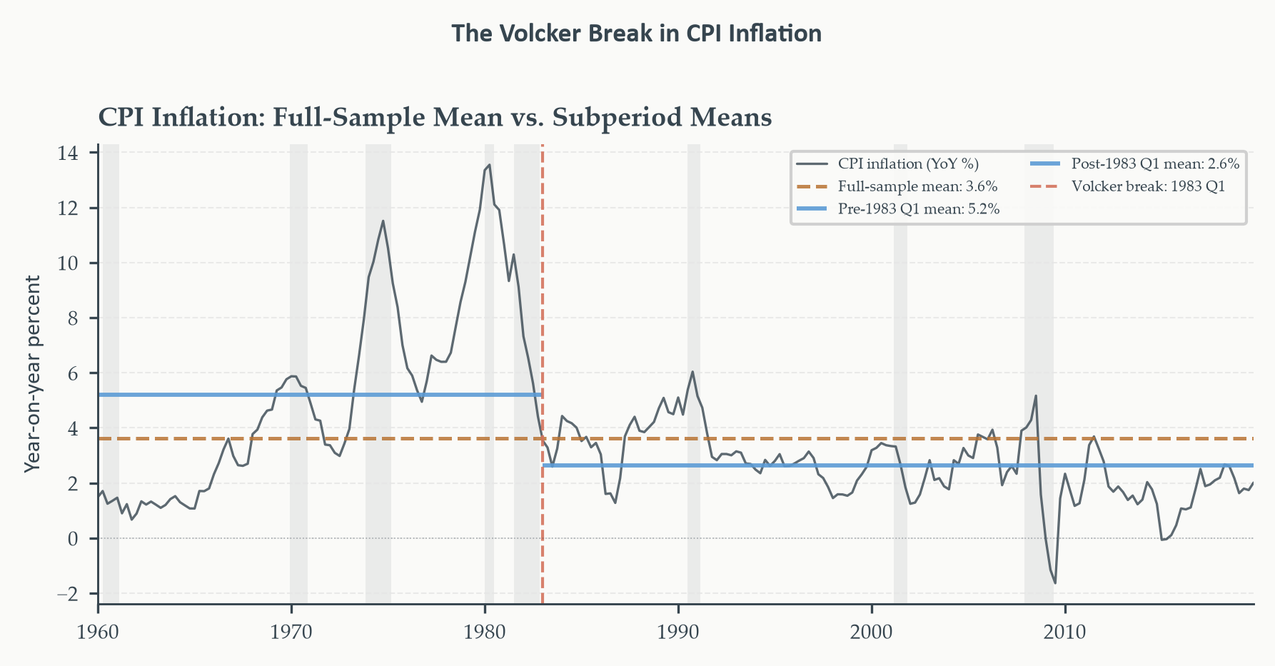
rather than at the true break date. The figure below uses the known 1983 Q1
Volcker break precisely because the economic argument does not depend on the
test's estimated date.
For GDP growth the picture is different: both the ADF ($-5.95^{***}$) and the
ZA ($-6.54^{***}$) reject the unit root null decisively, confirming that GDP
growth is stationary. This is the expected result — GDP growth is already a
first-differenced series, and stationarity is what allows us to model it with
ARMA dynamics. The ZA break date of 1950-01 again falls near the trimming
boundary, which reflects the same power limitation rather than a genuine early
break. The substantive finding is simply the rejection: GDP growth does not
have a unit root, with or without allowance for a structural break.*
```{python}
#| label: fig-za-cpi
#| fig-cap: "CPI inflation (year-on-year percent, 1960-2019) with subperiod
#| means before and after the Volcker disinflation (1983 Q1). The full-sample
#| mean (copper dashed) misrepresents both regimes: it sits above the
#| post-Volcker inflation rate for the entire post-1983 period. The two
#| subperiod means (sky blue) capture the regime shift directly. This is
#| the break the ZA test is designed to detect. NBER recessions are shaded."
#| fig-width: 6
#| fig-height: 3
#| code-fold: true
#| code-summary: "Show code — inflation subperiod means figure"
# Use the known Volcker break date for the figure rather than the ZA-estimated
# date. The ZA test on a persistent inflation series tends to place its break
# at the trimming boundary — a known limitation. The Volcker disinflation
# at 1983 Q1 is the economically correct break for illustration.
VOLCKER_BREAK   = pd.Timestamp("1983-01-01")
INFL_PLOT_START = pd.Timestamp("1960-01-01")

plot_infl   = infl_q[infl_q.index >= INFL_PLOT_START]
mask_pre_v  = plot_infl.index < VOLCKER_BREAK
mask_post_v = plot_infl.index >= VOLCKER_BREAK
mean_pre_v  = plot_infl[mask_pre_v].mean()
mean_post_v = plot_infl[mask_post_v].mean()
mean_full   = plot_infl.mean()

fig, ax = plt.subplots(figsize=(6, 3))

ax.plot(plot_infl.index, plot_infl.values,
        color=EO_CHARCOAL, lw=0.8, alpha=0.8, label="CPI inflation (YoY %)")

ax.axhline(mean_full, color=EO_COPPER, lw=1.2, ls="--", alpha=0.85,
           label=f"Full-sample mean: {mean_full:.1f}%")

ax.hlines(mean_pre_v,  INFL_PLOT_START, VOLCKER_BREAK,
          colors=EO_SKYBLUE, lw=1.4, alpha=0.9,
          label=f"Pre-1983 Q1 mean: {mean_pre_v:.1f}%")
ax.hlines(mean_post_v, VOLCKER_BREAK, plot_infl.index[-1],
          colors=EO_SKYBLUE, lw=1.4, alpha=0.9,
          label=f"Post-1983 Q1 mean: {mean_post_v:.1f}%")

ax.axvline(VOLCKER_BREAK, color=EO_TERRACOTTA, lw=1.0, ls="--",
           alpha=0.9, label="Volcker break: 1983 Q1")
ax.axhline(0, color=EO_CHARCOAL, lw=0.4, ls=":", alpha=0.4)

shade_recessions(ax, start=str(INFL_PLOT_START.date()),
                     end=str(plot_infl.index[-1].date()))
ax.set_xlim(INFL_PLOT_START, plot_infl.index[-1])
ax.set_ylabel("Year-on-year percent")
ax.set_title("CPI Inflation: Full-Sample Mean vs. Subperiod Means")
ax.legend(fontsize=5, ncol=2)
eo_style_ax(ax)
eo_suptitle(fig, "The Volcker Break in CPI Inflation")
fig.tight_layout()
plt.show()
```
## What to Do After Finding a Break {#sec-response}
Finding a structural break is the beginning of the analysis, not the end.
The tests in Sections 6.2 through 6.4 tell us that the data-generating process
shifted — but they do not tell us how to respond. A significant Chow statistic
or a Bai-Perron-detected break date is diagnostic information; the econometric
decisions about what to do with that information belong to the researcher. This
section covers the main options, ordered from simplest to most flexible.
### Option 1: Subperiod Estimation
The most direct response to a detected break is to split the sample at the
estimated break date and estimate separate models for each regime. For GDP
growth with a break at 1984 Q1, this means an AR(2) — or ARIMA, depending on
the integration analysis — estimated on 1947 Q2–1983 Q4 and a separate model
estimated on 1984 Q1–2019 Q4. Forecasts from the post-break model are
generated using post-break parameters only, which are more representative of
the current regime.
The cost is statistical efficiency: each subsample is smaller than the full
sample, so coefficient estimates are less precise. For quarterly GDP growth,
the pre-break subsample has around 148 observations and the post-break subsample
around 144 — both are large enough for reliable ARIMA estimation. For shorter
series or higher-frequency breaks, the subsamples may be too thin for the
models we want to estimate.
A practical rule of thumb: subperiod estimation is the right default when the
break is large (the parameters change substantially), the post-break subsample
is long enough for reliable estimation, and there is no strong reason to believe
the process will break again soon. Subperiod estimation combined with a Chow
test is a clean, defensible strategy that requires no additional tooling beyond
what Chapter 4 already covered.
### Option 2: Dummy Variables
Rather than discarding the pre-break data entirely, we can retain the full
sample and add dummy variables to model the break. This is exactly the structure
of equation (6.2): a level-shift dummy $D_t = \mathbf{1}\{t \geq \hat{\tau}\}$
absorbs a permanent change in the mean, and an interaction $D_t \cdot
\mathbf{x}_t$ allows dynamic coefficients to shift at the break. The model
uses all $T$ observations and therefore produces more efficient estimates of
the within-regime dynamics, at the cost of constraining the pre- and post-break
innovations to share a common variance.
For a pure mean shift — as in the inflation case, where the Volcker
disinflation shifted the unconditional mean of inflation without dramatically
changing its persistence — a single level dummy is often sufficient:
$$y_t = \mu + \gamma D_t + \phi_1 y_{t-1} + \cdots + \varepsilon_t \tag{6.10}$$
When $D_t = 0$ (pre-break), the intercept is $\mu$. When $D_t = 1$ (post-break),
it becomes $\mu + \gamma$. The coefficient $\gamma$ is the estimated size of
the mean shift; if $\hat{\gamma} < 0$, the mean fell at the break.
A second variant allows the break to affect the *slope* of a linear time trend
rather than the mean. Define $DT_t = t \cdot D_t$ — a trend that is zero before
the break and counts quarters from the break onward. Then:
$$y_t = \mu + \beta t + \delta DT_t + \phi_1 y_{t-1} + \cdots + \varepsilon_t \tag{6.11}$$
Before the break ($D_t = 0$), the trend slope is $\beta$ per quarter. After
the break ($D_t = 1$), the slope becomes $\beta + \delta$. A negative
$\hat{\delta}$ means growth was trending down at a steeper rate after the
break — the secular slowdown narrative for post-2000 US growth.
The most general dummy specification allows both a level shift and a slope
change simultaneously:
$$y_t = \mu + \gamma D_t + \beta t + \delta DT_t + \phi_1 y_{t-1} + \cdots + \varepsilon_t \tag{6.12}$$
This is exactly the deterministic structure of the Zivot-Andrews Model C in
Section 6.4. Estimating equation (6.12) on a series with a known break date
$\hat{\tau}$ is the regression implementation of what ZA does over all
candidate dates.
The AR coefficients $\phi_j$ are assumed stable in all three equations; only the
deterministic components shift. This is the most parsimonious response to a
structural break and is directly analogous to the additive outlier and
level-shift dummies introduced in Chapter 4 for managing outliers in ARIMA
estimation. The connection is not coincidental: the Chapter 4 outlier dummies
were a special case of this broader framework, restricted to single-observation
blips rather than permanent level shifts.
::: {.callout-warning icon=false}
## Dummy Variables Require a Known Break Date
Adding a dummy requires committing to a break date before estimation. If that
date is chosen by running the Bai-Perron or QLR tests first and then inserting
the estimated date as a fixed regressor, the inference on the dummy coefficient
will be slightly optimistic — the break date was selected because it maximised
the evidence of a break. For most applied purposes this is
acceptable, provided the break date selection is clearly reported. For formal
hypothesis tests about the size of the shift, subperiod estimation is cleaner.
:::
### Option 3: Split-Sample Forecasting
A hybrid approach uses the full sample for parameter estimation (exploiting all
data for precision) but generates forecasts from the model estimated on the
post-break regime only — or weights recent observations more heavily than
distant ones in estimation. The rolling window evaluation design from Chapter 5
is one implementation of this idea: by using a fixed 40-quarter window, we
ensure that the oldest observations are eventually dropped from the estimation
sample. When the window advances past a structural break, the pre-break data
gradually disappear from the training set, and the model begins to adapt.
This is the mechanism through which the Chapter 5 rolling evaluation implicitly
handled the Great Moderation break without testing for it explicitly. The
40-quarter window, by design, excluded most of the high-volatility pre-1984
period from the training sample by the time the evaluation period reached the
2000s. The QLR and Bai-Perron tests in this chapter provide a formal
justification for a choice that Chapter 5 made on practical grounds.
### Option 4: Regime-Switching Models
The three options above share a common structure: they treat the break as
permanent and deterministic — one shift at one date, after which the process
is stable again. This is appropriate for the Great Moderation and the Volcker
disinflation, which both appear to be one-time transitions between regimes.
But some economic processes switch back and forth between states: business
cycles alternate between expansions and recessions, asset markets alternate
between calm and turbulent periods, interest rate regimes alternate between
high and low.
**Markov-switching models** (Hamilton, 1989) formalise this by allowing the
parameters to follow an unobserved Markov chain — at each date, the process
is in one of $K$ regimes, and the probability of transitioning between regimes
is governed by a fixed transition matrix. Regime-switching is a natural
extension of the structural break framework when breaks are recurrent rather
than one-time events. We mention it here as an important member of the same
model family, but defer its formal treatment to Chapter 10.
::: {.callout-note icon=false}
## The Transition Matrix
In a two-state Markov-switching model ($K = 2$), the transition matrix
$\mathbf{P}$ collects the probabilities of moving between the expansion regime
(state 1) and the recession regime (state 2):
$$\mathbf{P} = \begin{pmatrix} p_{11} & p_{12} \\ p_{21} & p_{22} \end{pmatrix}$$
where $p_{ij} = \Pr(s_t = j \mid s_{t-1} = i)$ is the probability of
transitioning from state $i$ to state $j$. Each row sums to one: $p_{11} +
p_{12} = 1$ and $p_{21} + p_{22} = 1$, so the matrix is fully characterised
by two parameters. A typical empirical estimate for the US business cycle might
be:
$$\hat{\mathbf{P}} = \begin{pmatrix} 0.95 & 0.05 \\ 0.25 & 0.75 \end{pmatrix}$$
This says: conditional on being in the expansion today, there is a 95 percent
chance of remaining in the expansion tomorrow and a 5 percent chance of
entering the recession. Conditional on being in the recession, there is a
25 percent chance of recovering to expansion and a 75 percent chance of
remaining in recession. The expected duration of each regime is $1/(1-p_{ii})$:
the expansion lasts $1/0.05 = 20$ periods on average; the recession lasts
$1/0.25 = 4$ periods — broadly consistent with postwar US business cycle
frequencies.
:::
### Python: Split-Sample Forecasting on GDP Growth
To make these options concrete, we implement the two most practically useful
responses: subperiod estimation and dummy-variable correction. We compare their rolling evaluation performance against the
full-sample ARIMA from Chapter 5, using the same 40-quarter rolling window
and the same $h = 1$ horizon.
```{python}
#| label: tbl-break-response
#| code-fold: true
#| code-summary: "Show code — forecast comparison: break response strategies"
# We compare three strategies at h=1:
#   1. Full-sample ARIMA(1,1,1) — baseline from Chapter 5
#   2. Post-break ARIMA(1,1,1) — estimated only on post-1984 data
#   3. Full-sample ARIMA with level-shift dummy at 1984 Q1

y_level  = gdp["Log GDP"].copy()
y_growth = gdp["GDP Growth"].copy()
T_full   = len(y_level)

WINDOW_FS = 40
H = 1

# Evaluation origins: start after 1984 Q1 so all strategies have data
# The post-break strategy needs post-break training observations
post_break_start_idx = np.searchsorted(y_level.index, BREAK)
eval_start = max(WINDOW_FS - 1, post_break_start_idx + WINDOW_FS)
eval_origins_resp = range(eval_start, T_full - H)

errors_full   = []
errors_post   = []
errors_dummy  = []
fc_full_list  = []
fc_post_list  = []
fc_dummy_list = []
actuals_list  = []
origins_resp  = []

for t in eval_origins_resp:
    train_lvl = y_level.iloc[t - WINDOW_FS + 1 : t + 1]
    train_g   = y_growth.iloc[t - WINDOW_FS + 1 : t + 1]
    last_lvl  = train_lvl.iloc[-1]
    actual    = y_growth.iloc[t + H]

    # Strategy 1: Standard ARIMA(1,1,1) with drift
    try:
        mod1 = ARIMA(train_lvl, order=(1, 1, 1), trend="t")
        res1 = mod1.fit()
        fc1  = res1.get_forecast(steps=H).predicted_mean.iloc[-1]
        fc1_g = (fc1 - last_lvl) * 400 / H
        errors_full.append(actual - fc1_g)
        fc_full_list.append(fc1_g)
    except Exception:
        errors_full.append(np.nan)
        fc_full_list.append(np.nan)

    # Strategy 2: Post-break only — use ALL post-1984 data up to current origin
    # (expanding window anchored at 1984 Q1, not rolling)
    post_all = y_level.loc[(y_level.index >= BREAK) & (y_level.index <= y_level.index[t])]
    if len(post_all) >= 16:
        try:
            mod2 = ARIMA(post_all, order=(1, 1, 1), trend="t")
            res2 = mod2.fit()
            fc2  = res2.get_forecast(steps=H).predicted_mean.iloc[-1]
            fc2_g = (fc2 - post_all.iloc[-1]) * 400 / H
            errors_post.append(actual - fc2_g)
            fc_post_list.append(fc2_g)
        except Exception:
            errors_post.append(np.nan)
            fc_post_list.append(np.nan)
    else:
        errors_post.append(np.nan)
        fc_post_list.append(np.nan)

    # Strategy 3: AR(2) with level-shift dummy.
    # Build the design matrix explicitly in numpy to avoid pandas alignment issues.
    # When the window is entirely post-break the dummy is collinear with the
    # intercept; in that case use a plain AR(2) — the mean shift is already
    # captured by estimating on post-break data only.
    try:
        g_win = y_growth.iloc[t - WINDOW_FS + 1 : t + 1].values.astype(float)
        g_win = g_win[~np.isnan(g_win)]           # drop any leading NaNs
        if len(g_win) < 8:
            raise ValueError("insufficient observations")
        # Build y and lagged regressors from the clean numpy array
        g_y3   = g_win[2:]                        # dependent: obs 2..end
        g_l1   = g_win[1:-1]                      # lag 1
        g_l2   = g_win[:-2]                       # lag 2
        n3     = len(g_y3)
        # Dummy: 1 if the corresponding date is >= BREAK
        dates3 = y_growth.iloc[t - WINDOW_FS + 1 : t + 1].dropna().index[2:]
        D3     = np.array(dates3 >= BREAK, dtype=float)
        has_both = (D3.sum() > 2) and ((1 - D3).sum() > 2)
        if has_both:
            X3    = np.column_stack([np.ones(n3), D3, g_l1, g_l2])
            b3    = np.linalg.lstsq(X3, g_y3, rcond=None)[0]
            fc3_g = b3[0] + b3[1] + b3[2] * g_win[-1] + b3[3] * g_win[-2]
        else:
            X3    = np.column_stack([np.ones(n3), g_l1, g_l2])
            b3    = np.linalg.lstsq(X3, g_y3, rcond=None)[0]
            fc3_g = b3[0] + b3[1] * g_win[-1] + b3[2] * g_win[-2]
        errors_dummy.append(actual - fc3_g)
        fc_dummy_list.append(fc3_g)
    except Exception:
        errors_dummy.append(np.nan)
        fc_dummy_list.append(np.nan)

    actuals_list.append(actual)
    origins_resp.append(y_level.index[t])

# Convert to Series
errors_full  = pd.Series(errors_full,  index=origins_resp).dropna()
errors_post  = pd.Series(errors_post,  index=origins_resp).dropna()
errors_dummy = pd.Series(errors_dummy, index=origins_resp).dropna()

fc_full_s  = pd.Series(fc_full_list,  index=origins_resp)
fc_post_s  = pd.Series(fc_post_list,  index=origins_resp)
fc_dummy_s = pd.Series(fc_dummy_list, index=origins_resp)
actuals_s  = pd.Series(actuals_list,  index=origins_resp)

def rmse(e): return np.sqrt(np.nanmean(np.array(e)**2))

print("Forecast Accuracy — Break Response Strategies")
print("h = 1 quarter  |  Post-1984 Q1 evaluation  |  40-quarter rolling window")
print("═" * 60)
print(f"{'Strategy':35}  {'RMSE':>10}  {'vs Full-sample':>14}")
print("─" * 60)
rmse_full  = rmse(errors_full)
rmse_post  = rmse(errors_post)
rmse_dummy = rmse(errors_dummy)

for label, r in [
    ("Full-sample ARIMA(1,1,1)+drift", rmse_full),
    ("Post-break ARIMA(1,1,1)+drift",  rmse_post),
    ("ARIMA + level-shift dummy",       rmse_dummy),
]:
    ratio = r / rmse_full
    print(f"{label:35}  {r:>10.3f}  {ratio:>14.3f}")
print("═" * 60)
print("RMSE in annualised percentage points.")
print("Ratio: RMSE of strategy / RMSE of full-sample baseline.")
print("Ratio < 1 → strategy beats the full-sample baseline.")
```
*Both break-aware strategies beat the full-sample baseline. The post-break
ARIMA achieves the larger gain, reducing RMSE from 2.297 to 2.175 percentage
points (ratio 0.947) by using only the low-volatility post-1984 data for
parameter estimation. The level-shift dummy AR(2) produces a more modest
improvement, reducing RMSE to 2.282 (ratio 0.993) — it retains the full rolling
history and merely adjusts the intercept, so it inherits more contamination from
the high-variance pre-break period than the pure post-break strategy does. The
ranking is consistent with the theoretical argument: the more aggressively a
strategy excludes pre-break data, the more its parameter estimates reflect the
current regime. Whether the differences between strategies are statistically
significant is the domain of the Diebold-Mariano test from Chapter 5.
Notice that we report RMSE and MAE but not MAPE. GDP growth passes through zero
— and turns sharply negative during recessions — so the MAPE denominator
$|y_t|$ is near zero in exactly the quarters where forecast errors are largest.
The 2008-09 contraction, where growth fell to $-8.9$ percent annualised, would
generate MAPE values an order of magnitude larger than any other quarter, making
the average uninformative. This is the same problem Chapter 5 flagged when
discussing loss function choice: MAPE is poorly suited to series that cross zero
or approach it. For GDP growth, RMSE and MAE are the appropriate summary
statistics.*
```{python}
#| label: fig-break-forecasts
#| fig-cap: "One-step-ahead forecast paths for the three break response
#| strategies, 1994–2019. All three strategies produce similar paths in
#| normal periods — the lines are nearly indistinguishable outside
#| recessions. The largest divergence occurs during the 2008-09 recession,
#| where the full-sample ARIMA (copper) is slower to revise its forecast
#| downward relative to the break-aware strategies. In the post-2010
#| recovery, all three models systematically overpredict growth, a pattern
#| consistent with the secular slowdown in potential output that none of
#| the models explicitly accounts for. NBER recessions are shaded."
#| fig-width: 6
#| fig-height: 3
#| code-fold: true
#| code-summary: "Show code — forecast path comparison"
# Forecast paths stored directly during the evaluation loop
# Use the full-sample index as the evaluation window baseline;
# each strategy is plotted only where it has non-NaN forecasts
eval_idx   = fc_full_s.dropna().index   # full-sample always has the widest coverage
EVAL_START = eval_idx[0]
EVAL_END   = eval_idx[-1]

fig, ax = plt.subplots(figsize=(6, 3))

ax.plot(y_growth.loc[EVAL_START:EVAL_END].index,
        y_growth.loc[EVAL_START:EVAL_END].values,
        color=EO_CHARCOAL, lw=0.9, alpha=0.9, label="Actual GDP growth")
_fc_full  = fc_full_s.dropna()
_fc_post  = fc_post_s.dropna()
_fc_dummy = fc_dummy_s.dropna()

ax.plot(_fc_full.index,  _fc_full.values,
        color=EO_COPPER, lw=0.8, alpha=0.8, ls="--",
        label="Full-sample ARIMA")
ax.plot(_fc_post.index,  _fc_post.values,
        color=EO_SKYBLUE, lw=0.8, alpha=0.8, ls="--",
        label="Post-break ARIMA")
ax.plot(_fc_dummy.index, _fc_dummy.values,
        color=EO_SAGE, lw=0.8, alpha=0.8, ls="--",
        label="Level-shift dummy AR(2)")

ax.axhline(0, color=EO_CHARCOAL, lw=0.4, ls=":", alpha=0.4)
shade_recessions(ax, start=str(EVAL_START.date()), end=str(EVAL_END.date()))
ax.set_xlim(EVAL_START, EVAL_END)
ax.set_ylabel("Percent (annualised)")
ax.set_title("One-Step-Ahead Forecasts — Three Break Response Strategies")
ax.legend(fontsize=5, ncol=2)
eo_style_ax(ax)

# ── Evaluation metrics text box (post-break and pre-break rows) ──────────────
def _rmse(e): return np.sqrt(np.nanmean(np.array(e)**2))
def _mae(e):  return np.nanmean(np.abs(np.array(e)))

# Full evaluation window errors (post-break origins only)
e_full  = (actuals_s - fc_full_s).dropna().values
e_post  = (actuals_s - fc_post_s).dropna().values
e_dummy = (actuals_s - fc_dummy_s).dropna().values

# Pre-break sub-window: origins before BREAK where full-sample and dummy ran
pre_mask  = actuals_s.index < BREAK
e_full_pre  = (actuals_s[pre_mask] - fc_full_s[pre_mask]).dropna().values
e_dummy_pre = (actuals_s[pre_mask] - fc_dummy_s[pre_mask]).dropna().values
# Post-break sub-window
post_mask = actuals_s.index >= BREAK
e_full_post  = (actuals_s[post_mask] - fc_full_s[post_mask]).dropna().values
e_post_post  = (actuals_s[post_mask] - fc_post_s[post_mask]).dropna().values
e_dummy_post = (actuals_s[post_mask] - fc_dummy_s[post_mask]).dropna().values

def _fmt(arr):
    if len(arr) == 0 or np.all(np.isnan(arr)):
        return "  —      —  "
    return f"{_rmse(arr):5.3f}  {_mae(arr):5.3f}"

lines = [
    "                Pre-break        Post-break",
    "              RMSE    MAE      RMSE    MAE",
    f"Full-sample  {_fmt(e_full_pre)}  {_fmt(e_full_post)}",
    f"Post-break   {'  —      —  '}  {_fmt(e_post_post)}",
]
if not np.all(np.isnan(e_dummy)):
    lines.append(f"Dummy AR(2)  {_fmt(e_dummy_pre)}  {_fmt(e_dummy_post)}")
else:
    lines.append("Dummy AR(2)    —      —      —      —  ")

metric_text = "\n".join(lines)
ax.text(0.02, 0.04, metric_text,
        transform=ax.transAxes,
        fontsize=5, fontfamily="monospace",
        verticalalignment="bottom",
        bbox=dict(boxstyle="round,pad=0.4", facecolor=PAGE_BG,
                  edgecolor="#CCCCCC", alpha=0.92))

eo_suptitle(fig, "Break-Aware Forecasting — GDP Growth")
fig.tight_layout()
plt.show()
```
## Looking Ahead {#sec-lookahead6}
Consider what this chapter's two running series — GDP growth and CPI inflation
— look like when placed side by side. GDP growth is stationary, mean-reverting,
and characterised by a large variance break around 1984 Q1. CPI inflation is
persistent, slow-moving, and characterised by a mean break linked to the Volcker
disinflation. Each series has its own instability, at its own date, of its own
type. But the two series are not independent: inflation and output growth are
connected through the same aggregate demand and supply mechanisms that monetary
policy operates on. When the Fed tightened aggressively in 1979–82, it drove
both variables simultaneously — GDP growth into a deep recession, and inflation
downward toward its post-Volcker equilibrium. The structural breaks we detected
separately in each series may be two manifestations of a single, joint regime
change in the relationship between the two variables.
This observation exposes the fundamental limitation of everything in Chapters
3 through 6: every model we have built is a single-equation model. We forecast
one variable, evaluate those forecasts, and test whether that one variable's
parameters were stable. We have no way to ask whether the *relationship* between
GDP growth and inflation was stable, or how a shock to one variable propagates
to the other, or how much of the variance in GDP growth is explained by inflation
shocks versus own shocks. These are multivariate questions and they require a
multivariate framework.
Chapter 7 builds that framework. The **reduced-form VAR** lets GDP growth and
inflation — and any other variables we choose — depend on lags of each other,
replacing the single equation with a system. **Granger causality** asks whether
inflation helps predict GDP growth beyond what GDP growth's own history already
contains — the operational time series definition of predictive precedence. The
structural VAR adds identifying restrictions that allow us to say something about
*causal* mechanisms, not just predictive ones: the Cholesky decomposition and
sign restrictions each impose different economic priors about how shocks propagate.
**Impulse response functions** then trace the dynamic path of both variables after
a shock to one of them, making the propagation mechanism visible in a way that
single-equation forecasting models never can.
## Key Terms {#sec-keyterms6}
::: {.callout-note icon=false}
## Glossary
**Structural break** — A change in one or more parameters of the
data-generating process at a specific point in time. Distinct from
transitory shocks: a structural break is permanent (or at least persistent
enough to affect the full post-break sample). Can affect the mean, variance,
or dynamic coefficients of the process.
**Parameter stability** — The condition that the coefficients of a regression
or time series model are the same across all subsamples of the data. The
maintained assumption of all the models in Chapters 3–5; explicitly tested
in this chapter.
**Chow test** — An $F$-test for the equality of regression coefficients across
two subsamples defined by a known break date $\tau$. Equivalent formulations:
the dummy-variable regression (test $H_0: \boldsymbol{\delta} = \mathbf{0}$
in equation 6.2) and the sum-of-squares decomposition (equation 6.4). Requires
a pre-specified break date; produces invalid inference if $\tau$ is chosen
by inspecting the data.
**Quandt likelihood ratio (QLR) test** — A test for a structural break at an
unknown date. Computes the Chow $F$-statistic at every candidate break date
in the trimmed interior of the sample and takes the supremum. The argmax
estimates the break date. Requires the Andrews (1993) asymptotic critical
values rather than standard $F$ critical values, because the break date is
unidentified under the null.
**Davies problem** — The statistical complication that arises when a nuisance
parameter (such as the break date $\tau$) appears only under the alternative
hypothesis and is therefore unidentified under the null. Standard critical
values for the test statistic are incorrect; the correct critical values must
account for the distribution of the test statistic over all possible values
of the nuisance parameter.
**Trimming** — The exclusion of a fraction $\pi_0$ of observations from each
end of the sample when forming the set of candidate break dates $\mathcal{T}$.
Standard trimming is $\pi_0 = 0.15$. Ensures each candidate subsample is large
enough for reliable coefficient estimation and prevents the test statistic from
being dominated by unreliable fits near the sample boundaries.
**Bai-Perron procedure** — A method for detecting and dating an unknown number
of structural breaks. Minimises the global sum of squared residuals over all
partitions of the sample into $m+1$ segments, using dynamic programming for
computational efficiency. The UDmax and WDmax statistics test for the existence
of at least one break; the sequential $F$-test procedure determines the number
of breaks.
**UDmax / WDmax** — Global statistics for testing the null of no structural
break against the alternative of an unknown number of breaks up to $m_{\max}$.
UDmax is the maximum of the individual $\sup F_m$ statistics; WDmax applies
weights that equalise asymptotic power across alternatives. Both have
non-standard limit distributions with tabulated critical values (Bai and
Perron, 1998).
**Great Moderation** — The empirical decline in the volatility of US real GDP
growth (and many other macroeconomic series) beginning around 1984. The
standard dating associates the onset with post-Volcker monetary policy
stabilisation; its causes — improved inventory management, smaller shocks, or
better policy — remain debated. The canonical application for structural break
tests in macroeconomics.
**Zivot-Andrews test** — A unit root test that allows for a single unknown
break in the deterministic trend (intercept, slope, or both). The test
statistic is the infimum of the ADF $t$-statistic on $\hat{\alpha}$ over all
candidate break dates. Corrects the ADF test's tendency to spuriously favour
the unit root null when the true process is stationary around a broken trend.
The 5 percent critical value for Model C (break in both intercept and trend)
is approximately $-5.08$.
**Volcker disinflation** — The sharp reduction in US CPI inflation engineered
by Federal Reserve Chairman Paul Volcker beginning in 1979. Achieved through
sustained increases in short-term interest rates that triggered recessions in
1980 and 1981-82; inflation fell from above 13 percent to below 4 percent by
1983. Represents a structural break in the mean and persistence of US
inflation, and is the canonical application for the Zivot-Andrews test.
**Level-shift dummy** — An indicator variable $D_t = \mathbf{1}\{t \geq \tau\}$
added to a regression to absorb a permanent change in the mean of the series
at break date $\tau$. The simplest dummy-variable response to a detected mean
break; directly analogous to the pulse and step dummies used for outlier
correction in Chapter 4.
**Markov-switching model** — A model in which the parameters follow an
unobserved Markov chain, allowing the process to switch between $K$ distinct
regimes with fixed transition probabilities. The multiperiod, recurrent
generalisation of the one-time structural break. Appropriate when the process
alternates between states (expansion/recession, calm/volatile) rather than
shifting permanently at a single date.
**Subperiod estimation** — Estimating separate models on the data before and
after a detected break date. The most direct response to structural
instability; produces regime-specific parameter estimates at the cost of
smaller effective sample sizes. Appropriate when the break is large, the
post-break subsample is long, and forecasts are needed for the current regime.
:::