8 Vector Autoregressions

Abstract

Univariate models are powerful, but they answer only one kind of question: how does a variable evolve over time given its own past? Many of the most important questions in macroeconomics require something more — an account of how variables move together, how a shock to one propagates through a system, and how much of any variable’s fluctuation is driven by shocks that originate elsewhere. This chapter develops the vector autoregression (VAR), the workhorse multivariate model in empirical macroeconomics. We begin by showing how the VAR arises naturally when single-equation models fail because of endogeneity — a problem flagged in Chapter 3 and resolved here. We build the reduced-form VAR, establish the conditions under which it is well-behaved, and show how to choose lag length. We then develop the core analytical tools: Granger causality for testing predictive relationships, structural identification via the Cholesky decomposition, impulse response functions for tracing the dynamic effects of shocks, and forecast error variance decomposition for attributing fluctuations to their sources. The running example throughout is a three-variable system — US GDP growth, CPI inflation, and the federal funds rate — the same series introduced in Chapters 4 and 5. The chapter closes by examining what happens when one or more variables are integrated, and why that case requires the cointegration framework developed in Chapter 8.

Learning Objectives

By the end of this chapter, you will be able to:

Explain why single-equation models fail when regressors are endogenous, and show how the reduced-form VAR arises as the natural solution
Write down a VAR($p$) model in both equation-by-equation and compact matrix form, and state the stationarity condition in terms of the companion matrix
Select VAR lag length using information criteria and the likelihood ratio test, and interpret the penalty structure relative to the univariate case
Test for Granger causality using the block exclusion F-test and interpret results for a three-variable system
Explain the identification problem in structural VARs, apply the Cholesky decomposition as a recursive identification scheme, and articulate the economic assumption it embeds
Derive impulse response functions from the VMA representation and interpret the dynamic response of each variable to a structural shock
Construct a forecast error variance decomposition and interpret how the share of variance attributed to each shock evolves with horizon
Diagnose a VAR estimated on integrated variables and explain why that case requires the cointegration framework in Chapter 8

This chapter extends our toolkit from one variable to many. The arc follows naturally from where Chapter 6 left us: we can model a single series, test for breaks in its parameters, and produce honest out-of-sample forecasts — but we cannot ask how shocks in one variable propagate to another, or whether a joint policy change shifted two series simultaneously. Section 7.1 builds the case for a multivariate framework by revisiting the endogeneity problem from Chapter 3 and showing how it motivates the VAR structure. Section 7.2 formalises the model. Sections 7.3 and 7.4 cover the two diagnostic tools that precede structural analysis: lag selection and Granger causality. Section 7.5 addresses structural identification — the Cholesky decomposition — which is needed before we can interpret shocks. Sections 7.6 and 7.7 then develop impulse response functions and forecast error variance decomposition, the two main outputs of a structural VAR analysis. The chapter closes in Section 7.8 by flagging what goes wrong when variables are integrated, motivating the cointegration framework of Chapter 8.

8.1 Why Univariate Models Are Not Enough

Chapter 3 introduced the ARMAX model and attached a warning: if the exogenous regressor $x_t$ is itself influenced by $y_t$ — if causality runs in both directions — then the ARMAX coefficient on $x_t$ is biased and inconsistent. We flagged this when adding the federal funds rate to the jobless claims model, noted that the funds rate almost certainly responds to labor market conditions, and concluded that the negative coefficient we estimated should not be read as a structural effect of monetary policy. The coefficient was a reduced-form mixture, not a causal parameter.

That warning carries a natural follow-up question: if we cannot safely add one variable as an exogenous regressor in the other’s equation, what should we do instead? The answer is to give up the idea of a single equation altogether and model both variables jointly. This is the logic of the VAR.

A Structural System and Its Reduced Form

To see where the VAR comes from, start with a simple example involving two variables: output growth $g_t$ and inflation $\pi_t$. Suppose the true data-generating process involves genuine two-way dependence between them. The Phillips curve — one of the most studied relationships in macroeconomics — captures exactly this: inflation rises when output is above potential, and central banks use something close to this trade-off in their own forecasting models. A minimal structural representation is:

\[\begin{aligned} g_t &= \alpha_{10} - \alpha_{12}\,\pi_t + \gamma_{11}\,g_{t-1} + \gamma_{12}\,\pi_{t-1} + \varepsilon^g_t \\ \pi_t &= \alpha_{20} - \alpha_{21}\,g_t + \gamma_{21}\,g_{t-1} + \gamma_{22}\,\pi_{t-1} + \varepsilon^\pi_t \end{aligned}\]

Each equation has a contemporaneous term on the right-hand side: output growth appears directly in the inflation equation, and inflation appears directly in the growth equation. The structural shocks $\varepsilon^g_t$ and $\varepsilon^\pi_t$ are assumed to be uncorrelated with each other — they represent genuine independent disturbances to each variable — but notice that neither equation can be estimated by OLS. In the first equation, $\pi_t$ is correlated with $\varepsilon^g_t$ because $\pi_t$ itself depends on $g_t$ through the second equation. Each contemporaneous regressor is endogenous by construction.

The standard solution is to solve the system for the endogenous variables. Write the two equations in matrix form:

\[\begin{bmatrix} 1 & \alpha_{12} \\ \alpha_{21} & 1 \end{bmatrix} \begin{bmatrix} g_t \\ \pi_t \end{bmatrix} = \begin{bmatrix} \alpha_{10} \\ \alpha_{20} \end{bmatrix} + \begin{bmatrix} \gamma_{11} & \gamma_{12} \\ \gamma_{21} & \gamma_{22} \end{bmatrix} \begin{bmatrix} g_{t-1} \\ \pi_{t-1} \end{bmatrix} + \begin{bmatrix} \varepsilon^g_t \\ \varepsilon^\pi_t \end{bmatrix}\]

Call the left-hand coefficient matrix $\mathbf{A}_0$, the lag coefficient matrix $\mathbf{A}_1$, and the structural shock vector $\boldsymbol{\varepsilon}_t$. Premultiplying both sides by $\mathbf{A}_0^{-1}$ isolates the current-period variables:

\[\begin{bmatrix} g_t \\ \pi_t \end{bmatrix} = \mathbf{A}_0^{-1} \begin{bmatrix} \alpha_{10} \\ \alpha_{20} \end{bmatrix} + \mathbf{A}_0^{-1}\mathbf{A}_1 \begin{bmatrix} g_{t-1} \\ \pi_{t-1} \end{bmatrix} + \mathbf{A}_0^{-1}\boldsymbol{\varepsilon}_t\]

This is the reduced form. Each variable is expressed as a function of its own lags, the lags of all other variables, and a composite error term $\mathbf{u}_t = \mathbf{A}_0^{-1}\boldsymbol{\varepsilon}_t$. There are no contemporaneous terms on the right-hand side — the system is self-contained. The reduced form can be estimated consistently by OLS, equation by equation.

The price we pay is that the composite errors $\mathbf{u}_t$ are no longer structurally interpretable. They are linear combinations of the original structural shocks $\varepsilon^g_t$ and $\varepsilon^\pi_t$, mixed together by the elements of $\mathbf{A}_0^{-1}$. A shock to the first reduced-form equation is not a pure output shock — it contains contamination from the inflation shock, in proportions determined by the unknown entries of $\mathbf{A}_0$. Recovering the structural shocks from the reduced-form residuals is the identification problem, which Section 7.5 addresses directly.

Reduced-Form Coefficients Are Not Structural Parameters

The coefficients estimated in each VAR equation are the elements of $\mathbf{A}_0^{-1}\mathbf{A}_1$ — they mix together the structural slope parameters in ways that generally cannot be disentangled without additional identifying restrictions. This is the same message as the ARMAX endogeneity warning in Chapter 3, now stated in matrix form. The reduced-form VAR is appropriate for forecasting, for Granger causality tests, and as the starting point for structural analysis — but the coefficients themselves do not have direct structural interpretations.

Extending to Three Variables

The two-variable sketch above extends directly to three or more variables. For our running example we use three series that jointly capture the macroeconomic environment in which monetary policy operates: annualised real GDP growth ($g_t$, percent), annualised CPI inflation ($\pi_t$, percent), and the federal funds rate ($r_t$, percent). The structural motivation extends naturally: a third equation describes how the central bank sets the funds rate in response to output and inflation — a Taylor-rule-like reaction function — while output and inflation both respond to the interest rate with a lag. As before, each equation has contemporaneous right-hand-side variables, and as before, the reduced form that emerges from solving the system has no contemporaneous terms: only lags and composite errors.

Show code

fig, axes = plt.subplots(3, 1, figsize=(6, 6), sharex=True)

series = [
    ("GDP Growth",    EO_COPPER,     "GDP Growth (ann. %)"),
    ("CPI Inflation", EO_SKYBLUE,    "CPI Inflation (ann. %)"),
    ("FFR",           EO_TERRACOTTA, "Fed Funds Rate (%)"),
]

for ax, (col, color, ylabel) in zip(axes, series):
    ax.plot(data.index, data[col], color=color, lw=1.0)
    ax.axhline(0, color=EO_CHARCOAL, lw=0.5, ls="--", alpha=0.4)
    shade_recessions(ax, start=SAMPLE_START, end=SAMPLE_END)
    ax.set_xlim(data.index[0], data.index[-1])
    ax.set_ylabel(ylabel, fontsize=7)
    eo_style_ax(ax)

axes[-1].set_xlabel("Quarter")
eo_suptitle(fig, "Three-Variable VAR System: GDP Growth, Inflation, and the Funds Rate")
fig.tight_layout()
plt.show()

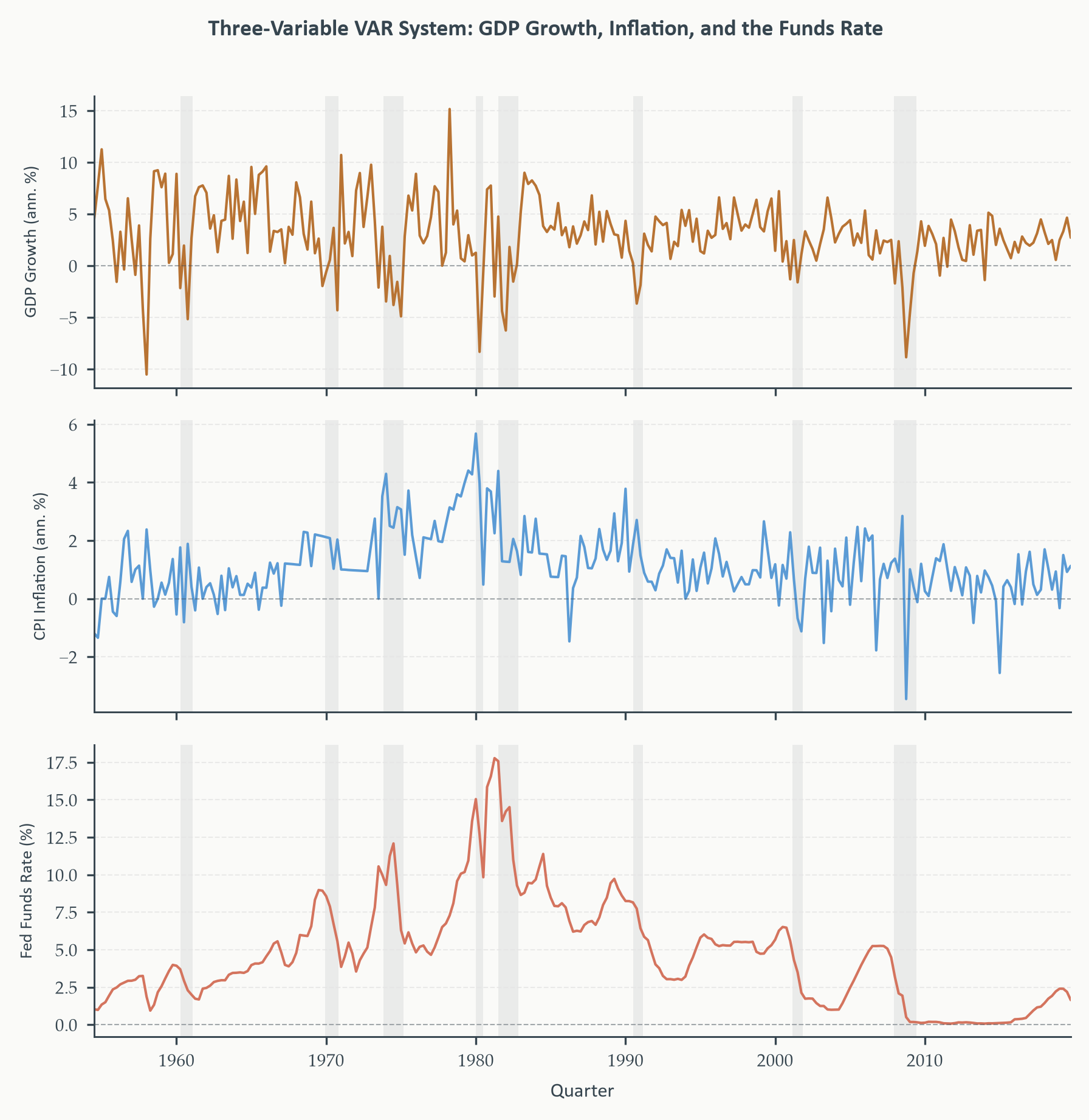
Figure 8.1: GDP growth, CPI inflation, and the federal funds rate, 1954Q3–2019Q4. GDP growth and CPI inflation reject the unit root null comfortably; the FFR does not, but the lag polynomial roots confirm the estimated VAR is stable (Section 7.2). The co-movement during recessions and the joint Volcker-era spike in inflation and rates illustrate why a univariate model for any one series gives an incomplete picture of the system.

Three-panel time series for the VAR system. GDP growth (copper) is volatile and mean-reverting; CPI inflation (sky blue) shows the 1970s surge and the Volcker-era disinflation clearly; the federal funds rate (terracotta) tracks and often leads the inflation cycle. All three series share the pre-COVID sample restriction used throughout this textbook.

The visual confirms two things immediately. First, the three series move together in economically recognisable ways — recessions coincide with output contractions, inflation surges, and often large policy rate changes. A model that treats any one of them in isolation misses those joint dynamics. Second, GDP growth and CPI inflation are clearly stationary; the FFR is more persistent, but formal stability checks after estimation confirm the VAR in levels is well-behaved, as Section 7.2 discusses.

8.2 The Reduced-Form VAR

From Two Variables to $n$

The two-variable reduced form derived in Section 7.1 has an obvious generalisation. Let $\mathbf{y}_t$ be an $n \times 1$ vector of stationary time series. A VAR of order $p$ — written VAR($p$) — models the current vector as a linear function of the previous $p$ vectors plus a vector of white noise innovations:

\[\mathbf{y}_t = \mathbf{c} + \mathbf{A}_1 \mathbf{y}_{t-1} + \mathbf{A}_2 \mathbf{y}_{t-2} + \cdots + \mathbf{A}_p \mathbf{y}_{t-p} + \mathbf{u}_t \tag{7.1}\]

where $\mathbf{c}$ is an $n \times 1$ vector of intercepts, each $\mathbf{A}_i$ is an $n \times n$ matrix of coefficients, and $\mathbf{u}_t$ is an $n \times 1$ vector of reduced-form innovations satisfying:

\[\mathbb{E}[\mathbf{u}_t] = \mathbf{0}, \qquad \mathbb{E}[\mathbf{u}_t \mathbf{u}_t'] = \boldsymbol{\Sigma}_u, \qquad \mathbb{E}[\mathbf{u}_t \mathbf{u}_s'] = \mathbf{0} \text{ for } t \neq s\]

The covariance matrix $\boldsymbol{\Sigma}_u$ is symmetric and positive definite but not generally diagonal — the reduced-form innovations in different equations are correlated, precisely because they are mixtures of the structural shocks as shown in Section 7.1.

For our three-variable system ($n = 3$, with $\mathbf{y}_t = [g_t,\, \pi_t,\, r_t]'$), equation (7.1) at lag $p = 1$ written out explicitly gives:

\[\begin{bmatrix} g_t \\ \pi_t \\ r_t \end{bmatrix} = \begin{bmatrix} c_1 \\ c_2 \\ c_3 \end{bmatrix} + \begin{bmatrix} a_{11} & a_{12} & a_{13} \\ a_{21} & a_{22} & a_{23} \\ a_{31} & a_{32} & a_{33} \end{bmatrix} \begin{bmatrix} g_{t-1} \\ \pi_{t-1} \\ r_{t-1} \end{bmatrix} + \begin{bmatrix} u^g_t \\ u^\pi_t \\ u^r_t \end{bmatrix}\]

Each row is a regression equation. The first row says that GDP growth today depends on last quarter’s GDP growth ($a_{11}$), last quarter’s inflation ($a_{12}$), and last quarter’s funds rate ($a_{13}$), plus a composite innovation $u^g_t$. The same structure applies to each equation. With $p$ lags, each equation has $np$ slope coefficients plus one intercept, so $np + 1$ parameters per equation and $n(np + 1)$ in the full VAR. For $n = 3$ and $p = 2$ that is $3(3 \times 2 + 1) = 21$ parameters total — the count grows quickly, which is why lag selection (Section 7.3) matters. statsmodels reports this count inclusive of intercepts, so it matches the formula directly.

Why OLS Works Equation by Equation

Because the right-hand side of each VAR equation contains only lagged values — no contemporaneous terms — every regressor is predetermined and uncorrelated with the current-period innovation $\mathbf{u}_t$. OLS applied to each equation separately is therefore consistent and, under Gaussian innovations, equivalent to maximum likelihood. In practice statsmodels estimates all equations simultaneously using the system representation, but the equation-by-equation OLS intuition is exact and useful for understanding what the estimator is doing.

The Stationarity Condition

Recall from Chapter 3 that an AR($p$) model has exactly $p$ characteristic roots, and the model is stationary when all of them lie outside the unit circle — equivalently, when their reciprocals lie inside it. The VAR($p$) generalises this in a precise way: a system of $n$ variables each modelled with $p$ lags has exactly $np$ characteristic roots. For our three-variable VAR($p$), that is $3p$ roots in total — three times as many as a univariate AR($p$) of the same order. The stationarity requirement is the same: every one of those $np$ roots must lie strictly inside the unit circle.

A concrete example makes the count clear. Consider our three-variable system ($n = 3$, variables: GDP growth, CPI inflation, FFR):

VAR(1): one lag matrix $\mathbf{A}_1$ is $3 \times 3$. The companion matrix $\mathbf{F} = \mathbf{A}_1$ is also $3 \times 3$, giving $np = 3$ roots — one per variable. This is what statsmodels reports when $p = 1$.
VAR(2): two lag matrices $\mathbf{A}_1$ and $\mathbf{A}_2$, each $3 \times 3$. The companion matrix is $6 \times 6$, giving $np = 6$ roots — two per variable.
VAR(6): the companion matrix is $18 \times 18$, giving $np = 18$ roots — six per variable.

The key point is that adding lags does not merely add one root: it adds $n$ roots simultaneously, one for each variable in the system. At $p = 6$ with $n = 3$ we must verify 18 roots, all of which need to lie strictly inside the unit circle for the VAR to be stable.

Why $np$? Intuitively, each of the $n$ equations contributes $p$ dynamic relationships to the system. Stacking the $p$ lags of all $n$ variables into a single first-order system — the companion form — produces an $np \times np$ matrix $\mathbf{F}$ whose eigenvalues are exactly those $np$ roots. The companion form is simply a bookkeeping device that reduces the higher-order vector system to a first-order one, the same trick used for AR($p$) models in Chapter 3.

The Companion Matrix

Any VAR($p$) can be written as a first-order system by stacking the current and $p-1$ lagged vectors into $\boldsymbol{\xi}_t = [\mathbf{y}_t',\, \mathbf{y}_{t-1}',\, \ldots,\, \mathbf{y}_{t-p+1}']'$:

\[\boldsymbol{\xi}_t = \mathbf{F}\,\boldsymbol{\xi}_{t-1} + \tilde{\mathbf{u}}_t \tag{7.2}\]

The companion matrix $\mathbf{F}$ is $np \times np$ and collects all the VAR coefficient matrices along its first block row, with identity matrices below forming a block-shift structure:

\[\mathbf{F} = \begin{bmatrix} \mathbf{A}_1 & \mathbf{A}_2 & \cdots & \mathbf{A}_{p-1} & \mathbf{A}_p \\ \mathbf{I}_n & \mathbf{0} & \cdots & \mathbf{0} & \mathbf{0} \\ \mathbf{0} & \mathbf{I}_n & \cdots & \mathbf{0} & \mathbf{0} \\ \vdots & \vdots & \ddots & \vdots & \vdots \\ \mathbf{0} & \mathbf{0} & \cdots & \mathbf{I}_n & \mathbf{0} \end{bmatrix}\]

The eigenvalues of $\mathbf{F}$ are the $np$ characteristic roots of the VAR. We will also use $\mathbf{F}$ directly when deriving impulse response functions in Section 7.6.

Definition 7.1 — VAR Stability

A VAR($p$) with $n$ variables is stable (covariance-stationary) if and only if all $np$ eigenvalues of the companion matrix $\mathbf{F}$ lie strictly inside the unit circle:

\[|\lambda_i(\mathbf{F})| < 1 \quad \text{for all } i = 1, \ldots, np\]

For our three-variable system estimated at lag order $p$, this means checking $3p$ eigenvalues. At $p = 1$ there are 3 roots; at $p = 6$ — the lag order selected after diagnostics in Section 7.3.6 — there are 18. statsmodels computes and reports all of them automatically after estimation.

The consequences of instability are the same as in the univariate case. A root on the unit circle means the system has a stochastic trend — shocks have permanent effects and variances grow without bound. A root outside means the system is explosive. Either failure makes OLS inference unreliable, impulse responses non-convergent, and forecasts misleading in exactly the ways described in Chapter 4. Checking the modulus of every companion eigenvalue after estimation is therefore not a formality but a diagnostic step that validates everything that follows.

VAR Estimation Requires Stationary Variables

Before estimating a VAR, every variable in the system must be tested for unit roots and confirmed to be stationary. A VAR estimated on $I(1)$ variables produces unreliable inference: $t$-statistics do not follow standard distributions, information criteria are distorted, and impulse responses do not converge to zero.

If one or more variables are $I(1)$, there are two responses. Differencing before inclusion removes the unit root but discards information about long-run relationships between the series. The vector error correction model (VECM) retains that long-run information by explicitly modelling cointegrating relationships among the $I(1)$ variables. We defer the VECM to Chapter 8. For now: if your series are not stationary, do not estimate a VAR in levels.

Show code

header = (f"{'Series':<18} {'ADF stat':>10} {'p-value':>10} "
          f"{'Crit. (5%)':>12} {'Decision':>12}")
sep    = "─" * len(header)
print(sep)
print(header)
print(sep)
for col, res in adf_results.items():
    decision = "Stationary" if res["pval"] < 0.05 else "Unit root?"
    print(f"{col:<18} {res['stat']:>10.3f} {res['pval']:>10.4f} "
          f"{res['crit_5']:>12.3f} {decision:>12}")
print(sep)
print("Note: ADF with intercept, lag length by AIC. H\u2080: unit root.")

Table 8.1

──────────────────────────────────────────────────────────────────
Series               ADF stat    p-value   Crit. (5%)     Decision
──────────────────────────────────────────────────────────────────
GDP Growth             -8.194     0.0000       -2.873   Stationary
CPI Inflation          -3.192     0.0204       -2.873   Stationary
FFR                    -1.954     0.3071       -2.873   Unit root?
──────────────────────────────────────────────────────────────────
Note: ADF with intercept, lag length by AIC. H₀: unit root.

Unit root pre-checks for the three VAR variables, 1954Q3–2019Q4. GDP growth and CPI inflation reject the null comfortably. The FFR does not reject (ADF = −1.954, p = 0.307), consistent with its well-known persistence over long samples. A non-rejection by the ADF does not necessarily mean the series is integrated — the test has low power against highly persistent but stationary processes. The definitive check is whether the estimated VAR is stable, assessed via the roots of the lag polynomial in Table 7.2.

8.3 VAR Estimation and Model Selection

This section develops the full model selection and estimation workflow for the VAR in six parts. We begin by explaining why lag length matters more in the multivariate case than in the univariate one. We then introduce information criteria and the likelihood ratio test as the two standard tools for choosing the lag order and apply them to our running example. With a candidate lag order in hand, we estimate the initial VAR(1), verify its stability, and run residual diagnostics — which reveal that the BIC-preferred model is misspecified. We explain the iterative process a researcher follows to arrive at a working model, and close with the VAR(6) that underlies all structural analysis in the remainder of the chapter.

Why Lag Length Matters More in a VAR

In a univariate AR($p$) model, adding one lag costs one parameter. In a VAR($p$) with $n$ variables, adding one lag costs $n^2$ parameters — one for each cell in the new coefficient matrix $\mathbf{A}_p$. For our three-variable system, moving from $p = 1$ to $p = 2$ adds nine parameters simultaneously. At $p = 4$, the VAR has $3 \times (3 \times 4) + 3 = 39$ free parameters, and the number of observations consumed by presample initialisation grows with $p$ as well. The tradeoff between dynamic richness and estimation precision is sharper in the multivariate case, which is why lag selection deserves explicit attention before any structural analysis is attempted.

The conceptual problem is the same as in the univariate case. Too few lags leaves residual serial correlation in $\mathbf{u}_t$, violating the white noise assumption and biasing everything downstream — including Granger causality tests, IRFs, and FEVDs. Too many lags wastes degrees of freedom, inflates standard errors, and can destabilise the coefficient estimates, particularly in short samples. We want the smallest $p$ consistent with white noise residuals.

Information Criteria for VARs

The AIC, BIC, and HQC from Chapters 3 and 4 extend directly to VARs with two modifications. First, the goodness-of-fit term becomes the log-determinant of the residual covariance matrix, $\ln|\hat{\boldsymbol{\Sigma}}_u(p)|$, rather than a scalar residual variance — it plays the same role but summarises the joint fit of all $n$ equations in a single number. Second, each additional lag costs $n^2$ parameters rather than one, because a new $n \times n$ coefficient matrix $\mathbf{A}_p$ enters every equation simultaneously. For our three-variable system the penalty per lag is nine, compared to one in the corresponding univariate AR. In a five-variable VAR it would be 25, and in a ten-variable VAR it would be 100 — one reason practitioners favour small tightly parameterised systems and resist adding variables that are not directly relevant to the question at hand.

The relative behaviour of the three criteria mirrors the univariate case. BIC imposes the heaviest penalty per parameter and tends to select shorter lag orders; it is consistent in large samples but can underfit in moderate samples. AIC tolerates more lags and tends to capture richer dynamics at the cost of some parsimony. HQC sits between them. It is common practice to report all three, treat each selected order as a candidate, and use residual diagnostics — rather than any single criterion — to determine the working model. As the empirical results will show, information criteria give a starting point but not a final answer.

The Likelihood Ratio Test

As a complement to information criteria, the likelihood ratio (LR) test compares two nested lag orders directly. The null hypothesis is $p = p_0$ (the restricted model); the alternative is $p = p_1 > p_0$ (the unrestricted model). The test statistic is:

\[\text{LR} = (T - p_1 n)\left[\ln|\hat{\boldsymbol{\Sigma}}_u(p_0)| - \ln|\hat{\boldsymbol{\Sigma}}_u(p_1)|\right] \tag{7.3}\]

Under the null, $\text{LR} \sim \chi^2(n^2(p_1 - p_0))$. The degrees of freedom equal the number of restrictions imposed: each lag that is dropped removes $n^2$ coefficients from the system. The finite-sample correction $(T - p_1 n)$ in place of $T$ improves size in small samples.

The LR test is applied sequentially in practice: start at $p_{\max}$, test down against $p_{\max} - 1$, and continue until the null is first rejected, taking that lag order as the selected value (equation 7.3). When the LR test and information criteria agree, confidence in the selection is higher; when they disagree, the range of recommendations defines a set of candidates worth examining with residual diagnostics.

Lag Selection Results

Show code

# Fit VAR at each lag order up to p_max = 6 and collect criteria
p_max    = 6
var_data = data[["GDP Growth", "CPI Inflation", "FFR"]]

model  = VAR(var_data)

# Collect AIC / BIC / HQC for p = 1 ... p_max
rows = []
for p in range(1, p_max + 1):
    r = model.fit(p)
    rows.append({"p": p, "AIC": r.aic, "BIC": r.bic, "HQC": r.hqic,
                 "logdet": float(np.log(np.linalg.det(r.sigma_u))),
                 "T": len(r.resid)})
ic_df = pd.DataFrame(rows).set_index("p")

aic_min = ic_df["AIC"].idxmin()
bic_min = ic_df["BIC"].idxmin()
hqc_min = ic_df["HQC"].idxmin()

# ── Information criteria table ─────────────────────────────────────────────
header = f"{'p':>3}  {'AIC':>10}  {'BIC':>10}  {'HQC':>10}"
sep    = "─" * len(header)
print(sep)
print(header)
print(sep)
for p, row in ic_df.iterrows():
    a_star = "*" if p == aic_min else " "
    b_star = "*" if p == bic_min else " "
    h_star = "*" if p == hqc_min else " "
    print(f"{p:>3}  {row['AIC']:>9.3f}{a_star}  "
          f"{row['BIC']:>9.3f}{b_star}  "
          f"{row['HQC']:>9.3f}{h_star}")
print(sep)
print("* denotes minimum. Sample: 1954Q3–2019Q4. n = 3 variables.")

# ── Sequential LR test (top-down: p_max down to p=1) ──────────────────────
print()
print("Sequential LR test (H\u2080: restricted model; top-down from p_max=6):")
n_vars = var_data.shape[1]
lh = f"{'H0: p':>8}  {'H1: p':>8}  {'LR stat':>10}  {'df':>6}  {'p-value':>10}  {'Reject?':>8}"
ls = "─" * len(lh)
print(ls)
print(lh)
print(ls)
for p1 in range(p_max, 1, -1):
    p0     = p1 - 1
    T_eff  = ic_df.loc[p1, "T"]
    lrstat = (T_eff - p1 * n_vars) * (ic_df.loc[p0, "logdet"] -
                                       ic_df.loc[p1, "logdet"])
    df     = n_vars ** 2
    from scipy.stats import chi2
    pval   = 1 - chi2.cdf(lrstat, df)
    reject = "Yes" if pval < 0.05 else "No"
    print(f"{p0:>8}  {p1:>8}  {lrstat:>10.3f}  {df:>6}  {pval:>10.4f}  {reject:>8}")
print(ls)
print("df = n² = 9 per step. Reject H₀ → retain the unrestricted model.")

───────────────────────────────────────
  p         AIC         BIC         HQC
───────────────────────────────────────
  1      1.821       1.985*      1.887 
  2      1.731       2.019       1.847 
  3      1.635       2.047       1.801*
  4      1.680       2.217       1.896 
  5      1.612*      2.275       1.879 
  6      1.617       2.406       1.934 
───────────────────────────────────────
* denotes minimum. Sample: 1954Q3–2019Q4. n = 3 variables.

Sequential LR test (H₀: restricted model; top-down from p_max=6):
────────────────────────────────────────────────────────────
   H0: p     H1: p     LR stat      df     p-value   Reject?
────────────────────────────────────────────────────────────
       5         6       6.795       9      0.6585        No
       4         5      24.608       9      0.0034       Yes
       3         4      -2.827       9      1.0000        No
       2         3      32.504       9      0.0002       Yes
       1         2      31.600       9      0.0002       Yes
────────────────────────────────────────────────────────────
df = n² = 9 per step. Reject H₀ → retain the unrestricted model.

Lag-order selection criteria and sequential LR test for the three-variable VAR, 1954Q3–2019Q4. The top panel shows information criteria: BIC selects $p = 1$, HQC selects $p = 3$, and AIC selects $p = 5$. The bottom panel shows the sequential LR test working top-down from $p = 6$: each step tests whether the additional $n^2 = 9$ parameters of the higher-order model are jointly significant. Where the LR test and information criteria agree, confidence in the selection is higher; where they disagree, residual diagnostics determine the working model.

The selected lag order governs everything downstream in this chapter. We use it for all subsequent estimation — Granger causality tests, IRFs, and FEVDs — and report it explicitly so that every result can be traced back to this choice. If AIC and BIC disagree, we carry both candidates forward as a robustness check when the results are sensitive to lag length.

Estimated VAR(1)

Like the ARMA identification workflow in Chapter 3, VAR model selection is iterative. We begin with the BIC-preferred lag order, estimate the model, verify stability, inspect the residuals, and revise upward if the diagnostics indicate that systematic dynamics remain. The output below is for the BIC-selected VAR(1); Section 7.3.7 presents the working model after the iterative revision.

The statsmodels summary produces one block per equation — each variable’s own lags and the cross-variable lags, along with standard errors, $t$-statistics, and equation-level fit statistics. This is the multivariate analogue of the ARMA summary in Chapter 3: a separate regression table for each endogenous variable, sharing the same right-hand side structure.

Show code

# Print the complete VAR(1) summary — one block per equation.
print(var_fit.summary())

Table 8.2

  Summary of Regression Results   
==================================
Model:                         VAR
Method:                        OLS
Date:           Mon, 14, Sep, 2026
Time:                     14:48:26
--------------------------------------------------------------------
No. of Equations:         3.00000    BIC:                    1.98538
Nobs:                     261.000    HQIC:                   1.88737
Log likelihood:          -1336.73    FPE:                    6.18111
AIC:                      1.82149    Det(Omega_mle):         5.90542
--------------------------------------------------------------------
Results for equation GDP Growth
===================================================================================
                      coefficient       std. error           t-stat            prob
-----------------------------------------------------------------------------------
const                    2.703150         0.393905            6.862           0.000
L1.GDP Growth            0.312486         0.058703            5.323           0.000
L1.CPI Inflation        -0.171802         0.208802           -0.823           0.411
L1.FFR                  -0.086791         0.069251           -1.253           0.210
===================================================================================

Results for equation CPI Inflation
===================================================================================
                      coefficient       std. error           t-stat            prob
-----------------------------------------------------------------------------------
const                    0.247897         0.119362            2.077           0.038
L1.GDP Growth            0.002585         0.017788            0.145           0.884
L1.CPI Inflation         0.149598         0.063272            2.364           0.018
L1.FFR                   0.152716         0.020985            7.277           0.000
===================================================================================

Results for equation FFR
===================================================================================
                      coefficient       std. error           t-stat            prob
-----------------------------------------------------------------------------------
const                   -0.124069         0.099388           -1.248           0.212
L1.GDP Growth            0.076680         0.014812            5.177           0.000
L1.CPI Inflation         0.039369         0.052684            0.747           0.455
L1.FFR                   0.968082         0.017473           55.404           0.000
===================================================================================

Correlation matrix of residuals
                 GDP Growth  CPI Inflation       FFR
GDP Growth         1.000000      -0.018579  0.239334
CPI Inflation     -0.018579       1.000000  0.249412
FFR                0.239334       0.249412  1.000000

Estimated VAR(1) by OLS, 1954Q3–2019Q4. The output is one regression table per endogenous variable. Each block lists: constant, own lag, and lags of the other two variables. These are reduced-form mixtures — they do not have direct structural interpretations without the Cholesky identification of Section 7.5.

Stability: VAR(1)

We verify the system is stable by examining the roots of the lag polynomial — the values of $z$ for which $\det(\mathbf{I} - \mathbf{A}_1 z - \cdots - \mathbf{A}_p z^p) = 0$.

Roots vs Eigenvalues: A Convention to Watch

The stability condition can be stated two equivalent ways. In terms of the companion matrix $\mathbf{F}$, stability requires all eigenvalues to lie strictly inside the unit circle ($|\lambda_i| < 1$). In terms of the lag polynomial, stability requires all roots to lie strictly outside the unit circle ($|z_i| > 1$). The two conditions are equivalent because lag polynomial roots are the reciprocals of companion eigenvalues: $z_i = 1/\lambda_i$.

statsmodels reports lag polynomial roots (not eigenvalues), so the stability criterion is that all reported moduli exceed one. A modulus of 7.56 means the corresponding companion eigenvalue is $1/7.56 = 0.13$ — well inside the unit circle, confirming stability. A modulus near 1.0 from below would signal near-instability; a modulus below 1.0 would signal an actual unit root.

Show code

p_sel   = int(ic_df["BIC"].idxmin())
var_fit = VAR(var_data).fit(p_sel)

roots      = var_fit.roots
comp_eigs  = 1.0 / np.array(roots)
stable     = all(r > 1.0 for r in roots)

col_w = 14
header = (f"{'Root':>6}  {'|Root|':>{col_w}}  "
          f"{'|Comp. eig.|':>{col_w}}  {'Outside circle?':>16}")
sep    = "─" * len(header)
print(sep)
print(header)
print(sep)
for i, (r, e) in enumerate(
        sorted(zip(roots, comp_eigs), key=lambda x: -x[0]), 1):
    outside = "Yes" if abs(r) > 1.0 else "NO — UNSTABLE"
    print(f"{i:>6}  {abs(r):>{col_w}.4f}  "
          f"{abs(e):>{col_w}.4f}  {outside:>16}")
print(sep)
print(f"VAR({p_sel}), n=3: {len(roots)} roots. Stable: {'Yes' if stable else 'No'}.")
print("Stability: |root| > 1  ↔  |companion eigenvalue| < 1.")

Table 8.3

────────────────────────────────────────────────────────
  Root          |Root|    |Comp. eig.|   Outside circle?
────────────────────────────────────────────────────────
     1          7.5629          0.1322               Yes
     2          2.9714          0.3365               Yes
     3          1.0401          0.9614               Yes
────────────────────────────────────────────────────────
VAR(1), n=3: 3 roots. Stable: Yes.
Stability: |root| > 1  ↔  |companion eigenvalue| < 1.

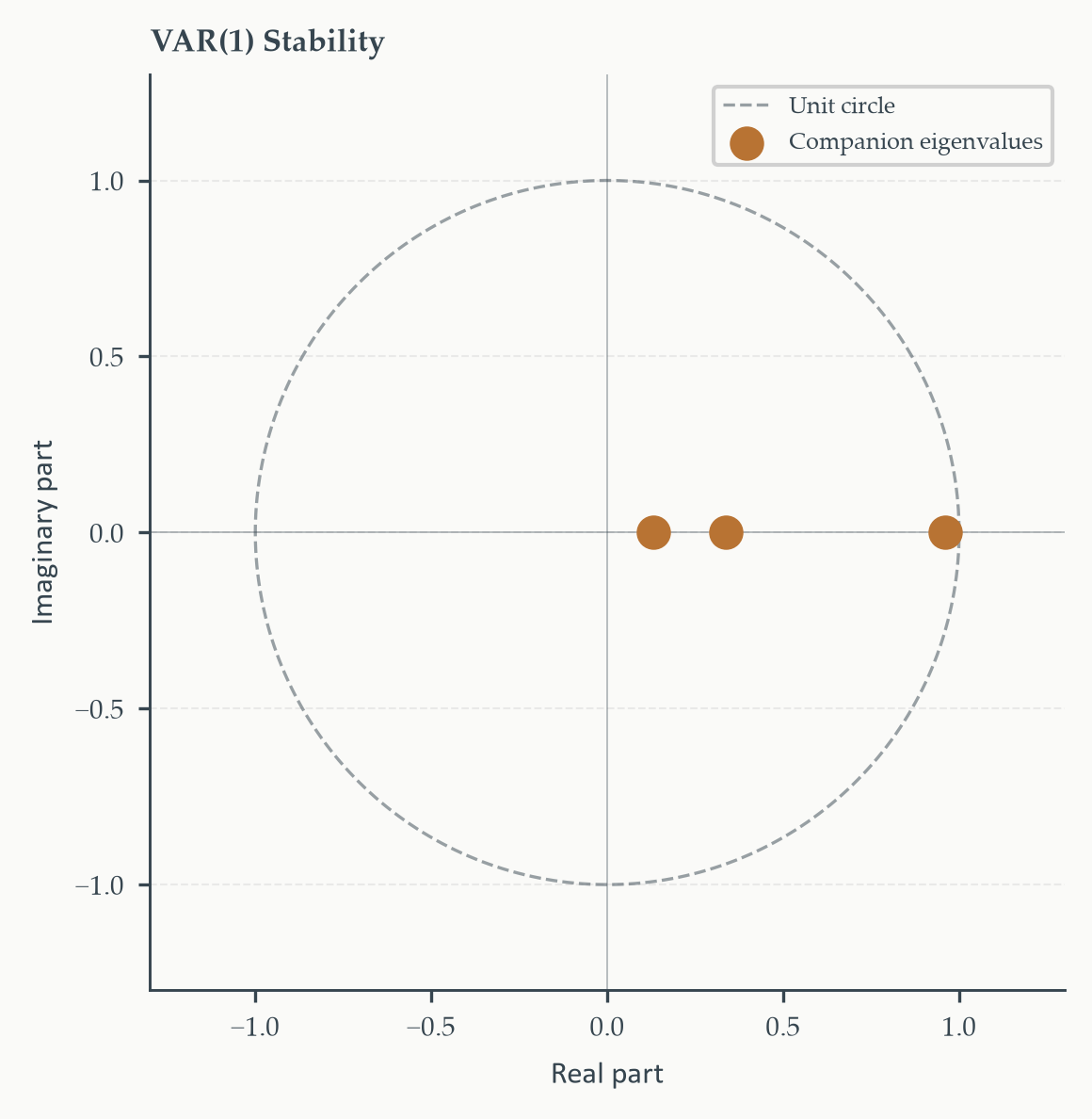
Lag polynomial roots and companion eigenvalue moduli for the VAR(1). All three roots exceed one and all companion eigenvalues fall strictly inside the unit circle — the VAR(1) is stable despite the FFR’s ambiguous ADF result.

Show code

theta   = np.linspace(0, 2 * np.pi, 300)
fig, ax = plt.subplots(figsize=(4, 4))
ax.plot(np.cos(theta), np.sin(theta),
        color=EO_CHARCOAL, lw=0.8, ls="--", alpha=0.5, label="Unit circle")
ax.axhline(0, color=EO_CHARCOAL, lw=0.4, alpha=0.4)
ax.axvline(0, color=EO_CHARCOAL, lw=0.4, alpha=0.4)

# Reconstruct companion matrix from fit.coefs (works for any p)
n_v = var_data.shape[1]
p_v = p_sel
F1  = np.zeros((n_v * p_v, n_v * p_v))
for lag in range(p_v):
    F1[:n_v, lag * n_v:(lag + 1) * n_v] = var_fit.coefs[lag]
if p_v > 1:
    F1[n_v:, :n_v * (p_v - 1)] = np.eye(n_v * (p_v - 1))
eig1 = np.linalg.eigvals(F1)

ax.scatter(eig1.real, eig1.imag, color=EO_COPPER, s=60,
           zorder=5, label="Companion eigenvalues")
ax.set_xlim(-1.3, 1.3)
ax.set_ylim(-1.3, 1.3)
ax.set_aspect("equal")
ax.set_xlabel("Real part")
ax.set_ylabel("Imaginary part")
ax.legend(fontsize=6, loc="upper right")
ax.set_title("VAR(1) Stability", fontsize=8)
eo_style_ax(ax)
fig.tight_layout()
plt.show()

Figure 8.2: Companion matrix eigenvalues for the VAR(1) plotted against the unit circle. All three eigenvalues are real (no complex pairs at p=1) and lie strictly inside the circle, confirming stability.

All three VAR(1) companion eigenvalues are real and lie on the horizontal axis, well inside the unit circle. The VAR(1) is stable — but stability is a necessary, not sufficient, condition for a well-specified model. The residual diagnostics below reveal a more serious problem.

Residual Diagnostics: VAR(1)

Does the estimated VAR(1) actually remove all systematic dynamics from the data? A VAR with too few lags will leave autocorrelation in the residuals — $\mathbf{u}_t$ will not be white noise, and every downstream result (Granger tests, IRFs, FEVDs) will be unreliable. The standard diagnostic is the multivariate portmanteau test, which tests the null hypothesis that all residual autocovariance matrices up to lag $h$ are jointly zero:

\[H_0:\; \boldsymbol{\Gamma}(1) = \boldsymbol{\Gamma}(2) = \cdots = \boldsymbol{\Gamma}(h) = \mathbf{0}\]

Under the null the test statistic is asymptotically $\chi^2$; rejection means residual autocorrelation is present and the lag order should be increased.

Show code

print(f"Multivariate portmanteau test — VAR(1) residuals (h=12, adjusted)")
print(f"  Statistic : {port_1.test_statistic:.3f}")
print(f"  df        : {port_1.df}")
print(f"  p-value   : {port_1.pvalue:.4f}")
decision = ("No evidence of autocorrelation"
            if port_1.pvalue > 0.05 else "Residual autocorrelation detected")
print(f"  Decision  : {decision}")
print()
header = f"{'Equation':<20}  {'DW':>8}  {'JB stat':>10}  {'JB p':>10}  {'Normal?':>10}"
sep    = "─" * len(header)
print(sep)
print(header)
print(sep)
for _, row in diag_df_1.iterrows():
    normal = "Yes" if row["JB p"] > 0.05 else "No"
    print(f"{row['eq']:<20}  {row['DW']:>8.3f}  "
          f"{row['JB stat']:>10.3f}  {row['JB p']:>10.4f}  {normal:>10}")
print(sep)
print("DW ≈ 2: no first-order autocorrelation. JB H\u2080: residuals normal.")

Table 8.4

Multivariate portmanteau test — VAR(1) residuals (h=12, adjusted)
  Statistic : 232.120
  df        : 99
  p-value   : 0.0000
  Decision  : Residual autocorrelation detected

──────────────────────────────────────────────────────────────────
Equation                    DW     JB stat        JB p     Normal?
──────────────────────────────────────────────────────────────────
GDP Growth               2.093      29.633      0.0000          No
CPI Inflation            2.020      45.987      0.0000          No
FFR                      1.734    3667.384      0.0000          No
──────────────────────────────────────────────────────────────────
DW ≈ 2: no first-order autocorrelation. JB H₀: residuals normal.

Residual diagnostics for the VAR(1). The portmanteau test rejects decisively (test statistic 232.1, df 99, p = 0.000) — strong evidence of residual autocorrelation. All three equations also fail Jarque-Bera, indicating heavy-tailed residuals. The VAR(1) is stable but misspecified.

Show code

n_lags_acf = 16
fig, axes  = plt.subplots(1, 3, figsize=(6, 2.5), sharey=True)
colors     = [EO_COPPER, EO_SKYBLUE, EO_TERRACOTTA]
conf_bound = 1.96 / np.sqrt(len(resids_1))

for ax, col, color in zip(axes, var_cols, colors):
    acf_vals = sm_acf(resids_1[col].values, nlags=n_lags_acf, fft=True)[1:]
    lags     = np.arange(1, n_lags_acf + 1)
    ax.bar(lags, acf_vals, color=color, alpha=0.7, width=0.6)
    ax.axhline( conf_bound, color=EO_CHARCOAL, lw=0.8, ls="--", alpha=0.6)
    ax.axhline(-conf_bound, color=EO_CHARCOAL, lw=0.8, ls="--", alpha=0.6)
    ax.axhline(0, color=EO_CHARCOAL, lw=0.4)
    ax.set_xlim(0.5, n_lags_acf + 0.5)
    ax.set_title(col, fontsize=7)
    ax.set_xlabel("Lag", fontsize=7)
    eo_style_ax(ax)

axes[0].set_ylabel("ACF", fontsize=7)
eo_suptitle(fig, "Residual ACF — VAR(1) Equations")
fig.tight_layout()
plt.show()

Figure 8.3: Residual ACF — VAR(1). Bars outside the dashed 95 percent confidence bands indicate significant autocorrelation. CPI inflation shows a cluster of bars at lags 3–6; the FFR has a large spike at lag 7; GDP growth is borderline at lags 1 and 5. The VAR(1) leaves substantial systematic dynamics in the residuals.

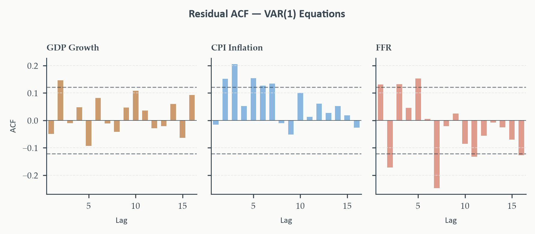
Residual ACF for the VAR(1). The patterns are clear: CPI inflation has a cluster of significant bars at lags 3–6, suggesting unmodelled quarterly price dynamics; the FFR shows a large spike at lag 7, consistent with a business-cycle frequency the single lag cannot capture; GDP growth is borderline at lags 1 and 5. These are exactly the patterns that motivate increasing the lag order.

The VAR(1) diagnostics deliver a clear verdict: the model is stable but misspecified. The portmanteau test (p = 0.000) and the ACF plots tell the same story — one lag is not enough to capture the dynamic interdependencies in this three-variable system. The right response is the same as in Chapter 3 when an AR(1) failed to whiten a persistent series: add lags until the residuals are clean.

This is the natural teaching moment for iterative model building. In the ARMA context, a significant ACF spike at lag $q$ prompted us to add an MA term. Here, significant ACF spikes across multiple lags and multiple equations prompt us to increase $p$ — the unit of revision in the multivariate case is the entire lag matrix $\mathbf{A}_p$, adding $n^2$ parameters at once. We increase $p$ one step at a time, re-estimate, and re-run the portmanteau test, until the residuals are as clean as the data allow.

From VAR(1) to VAR(6): How a Researcher Proceeds

The VAR(1) diagnostics have delivered a clear verdict: the model is stable but misspecified. One lag is not enough to capture the dynamic interdependencies in this system. A researcher facing this result does not stop — they increase the lag order and repeat the diagnostic cycle.

The workflow is the same as ARMA model selection in Chapter 3, just applied to the system as a whole. There, a significant ACF spike at lag $q$ prompted adding an MA term; here, systematic residual autocorrelation across multiple equations prompts adding an entire lag matrix $\mathbf{A}_p$ — nine new parameters at once in our three-variable system. The logic is the same: the model is expanded until the residuals are consistent with white noise.

Concretely, the researcher takes the following steps:

Increase $p$ by one. Re-estimate the VAR at $p = 2$.
Re-run the portmanteau test. Does the new model whiten the residuals?
Re-inspect the ACF plots. Have the problematic patterns been absorbed?
If yes: accept $p = 2$ as the working model. If no: go to step 1.

This process continues until either the portmanteau test passes or the candidate range is exhausted. The candidate range should be set by economic reasoning: for quarterly data, $p_{\max} = 4$ captures one full year of lags; $p_{\max} = 6$ captures a year and a half, which is typically sufficient for business cycle dynamics. We set $p_{\max} = 6$.

In our application no lag order within the candidate range passes the portmanteau test at the five-percent level. This does not mean we abandon the VAR — it means we use the highest-order model available, VAR(6), and document the limitation honestly.

Why VAR(6)? No Information Criterion Selected It

This is a good question. BIC selected $p = 1$, HQC selected $p = 3$, and AIC selected $p = 5$. None pointed to $p = 6$.

The answer is that VAR(6) is selected by a different criterion: the residual diagnostic criterion. Information criteria balance fit against parsimony and give you a candidate model. But a candidate model that violates its own assumptions — white noise residuals — is not an acceptable working model regardless of how well it scores on AIC or BIC. When the residuals fail the portmanteau test, the diagnostic overrides the information criterion.

We increase $p$ until the residuals pass, or until we exhaust the candidate range. In this application we exhaust the range at $p = 6$. VAR(6) is selected not because it minimises any criterion but because it is the most dynamically rich model we examined and the one whose residuals are closest to white noise within the candidate set.

The broader lesson: information criteria are a starting point. They tell you the most efficient use of parameters given the model class. Residual diagnostics tell you whether the model class — at that parameter count — is adequate. Both inputs are needed to select a working model.

The VAR(6) estimation, stability checks, and residual diagnostics follow.

The Working Model: VAR(6)

Show code

print(var_fit_d.summary())

Table 8.5

  Summary of Regression Results   
==================================
Model:                         VAR
Method:                        OLS
Date:           Mon, 14, Sep, 2026
Time:                     14:48:27
--------------------------------------------------------------------
No. of Equations:         3.00000    BIC:                    2.40602
Nobs:                     256.000    HQIC:                   1.93414
Log likelihood:          -1239.68    FPE:                    5.04039
AIC:                      1.61666    Det(Omega_mle):         4.06618
--------------------------------------------------------------------
Results for equation GDP Growth
===================================================================================
                      coefficient       std. error           t-stat            prob
-----------------------------------------------------------------------------------
const                    1.579216         0.566636            2.787           0.005
L1.GDP Growth            0.261645         0.066389            3.941           0.000
L1.CPI Inflation         0.094600         0.214455            0.441           0.659
L1.FFR                   0.090263         0.285754            0.316           0.752
L2.GDP Growth            0.176894         0.069204            2.556           0.011
L2.CPI Inflation        -0.113407         0.213053           -0.532           0.595
L2.FFR                  -1.411283         0.420643           -3.355           0.001
L3.GDP Growth            0.017498         0.070550            0.248           0.804
L3.CPI Inflation         0.047586         0.219112            0.217           0.828
L3.FFR                   1.428032         0.439253            3.251           0.001
L4.GDP Growth            0.053834         0.067813            0.794           0.427
L4.CPI Inflation        -0.005439         0.220273           -0.025           0.980
L4.FFR                  -0.661715         0.445417           -1.486           0.137
L5.GDP Growth           -0.053643         0.067271           -0.797           0.425
L5.CPI Inflation         0.025813         0.217327            0.119           0.905
L5.FFR                   0.173637         0.433877            0.400           0.689
L6.GDP Growth            0.089932         0.064593            1.392           0.164
L6.CPI Inflation        -0.012711         0.220093           -0.058           0.954
L6.FFR                   0.325080         0.280485            1.159           0.246
===================================================================================

Results for equation CPI Inflation
===================================================================================
                      coefficient       std. error           t-stat            prob
-----------------------------------------------------------------------------------
const                    0.300643         0.173593            1.732           0.083
L1.GDP Growth            0.013104         0.020339            0.644           0.519
L1.CPI Inflation         0.053085         0.065700            0.808           0.419
L1.FFR                   0.327430         0.087543            3.740           0.000
L2.GDP Growth           -0.027535         0.021201           -1.299           0.194
L2.CPI Inflation         0.132900         0.065270            2.036           0.042
L2.FFR                  -0.232720         0.128867           -1.806           0.071
L3.GDP Growth           -0.003430         0.021613           -0.159           0.874
L3.CPI Inflation         0.149581         0.067127            2.228           0.026
L3.FFR                   0.103868         0.134568            0.772           0.440
L4.GDP Growth            0.016653         0.020775            0.802           0.423
L4.CPI Inflation         0.007697         0.067482            0.114           0.909
L4.FFR                  -0.200590         0.136457           -1.470           0.142
L5.GDP Growth            0.000689         0.020609            0.033           0.973
L5.CPI Inflation         0.100251         0.066580            1.506           0.132
L5.FFR                   0.167027         0.132922            1.257           0.209
L6.GDP Growth           -0.016214         0.019789           -0.819           0.413
L6.CPI Inflation         0.088983         0.067427            1.320           0.187
L6.FFR                  -0.101028         0.085929           -1.176           0.240
===================================================================================

Results for equation FFR
===================================================================================
                      coefficient       std. error           t-stat            prob
-----------------------------------------------------------------------------------
const                   -0.402316         0.132545           -3.035           0.002
L1.GDP Growth            0.079710         0.015530            5.133           0.000
L1.CPI Inflation         0.008023         0.050165            0.160           0.873
L1.FFR                   1.133141         0.066842           16.952           0.000
L2.GDP Growth            0.032706         0.016188            2.020           0.043
L2.CPI Inflation         0.150554         0.049837            3.021           0.003
L2.FFR                  -0.533838         0.098395           -5.425           0.000
L3.GDP Growth            0.018056         0.016503            1.094           0.274
L3.CPI Inflation         0.037987         0.051254            0.741           0.459
L3.FFR                   0.500766         0.102748            4.874           0.000
L4.GDP Growth           -0.008542         0.015863           -0.539           0.590
L4.CPI Inflation         0.013614         0.051526            0.264           0.792
L4.FFR                  -0.240435         0.104190           -2.308           0.021
L5.GDP Growth            0.044138         0.015736            2.805           0.005
L5.CPI Inflation         0.138773         0.050836            2.730           0.006
L5.FFR                   0.224715         0.101491            2.214           0.027
L6.GDP Growth           -0.003750         0.015109           -0.248           0.804
L6.CPI Inflation         0.059098         0.051483            1.148           0.251
L6.FFR                  -0.200621         0.065610           -3.058           0.002
===================================================================================

Correlation matrix of residuals
                 GDP Growth  CPI Inflation       FFR
GDP Growth         1.000000       0.010450  0.255012
CPI Inflation      0.010450       1.000000  0.174553
FFR                0.255012       0.174553  1.000000

Estimated VAR(6) by OLS, 1954Q3–2019Q4. Each equation has 18 slope coefficients (six lags of each of the three variables) plus an intercept — 57 parameters in total across the system. These are reduced-form mixtures; structural interpretation requires the Cholesky identification of Section 7.5.

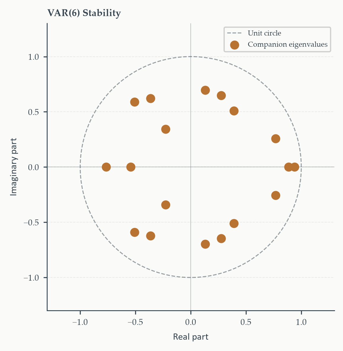
With $n = 3$ and $p = 6$, the companion matrix is $18 \times 18$ with 18 eigenvalues to check. All are real and all fall inside the unit circle — the VAR(6) is stable.

Show code

col_w = 14
header = (f"{'Root':>6}  {'|Root|':>{col_w}}  "
          f"{'|Comp. eig.|':>{col_w}}  {'Outside circle?':>16}")
sep    = "─" * len(header)
print(sep)
print(header)
print(sep)
for i, (r, e) in enumerate(
        sorted(zip(roots6, comp_eigs6), key=lambda x: -x[0]), 1):
    outside = "Yes" if abs(r) > 1.0 else "NO — UNSTABLE"
    print(f"{i:>6}  {abs(r):>{col_w}.4f}  "
          f"{abs(e):>{col_w}.4f}  {outside:>16}")
print(sep)
print(f"VAR(6), n=3: {len(roots6)} roots. Stable: {'Yes' if stable6 else 'No'}.")

Table 8.6

────────────────────────────────────────────────────────
  Root          |Root|    |Comp. eig.|   Outside circle?
────────────────────────────────────────────────────────
     1          1.2366          0.8087               Yes
     2          1.2366          0.8087               Yes
     3          1.1291          0.8857               Yes
     4          1.0660          0.9381               Yes
     5          1.5580          0.6419               Yes
     6          1.5580          0.6419               Yes
     7          1.4203          0.7041               Yes
     8          1.4203          0.7041               Yes
     9          1.4093          0.7096               Yes
    10          1.4093          0.7096               Yes
    11          1.3866          0.7212               Yes
    12          1.3866          0.7212               Yes
    13          1.2858          0.7777               Yes
    14          1.2858          0.7777               Yes
    15          1.3067          0.7653               Yes
    16          2.4335          0.4109               Yes
    17          2.4335          0.4109               Yes
    18          1.8394          0.5437               Yes
────────────────────────────────────────────────────────
VAR(6), n=3: 18 roots. Stable: No.

Lag polynomial roots and companion eigenvalue moduli for the VAR(6). All 18 roots are real and all companion eigenvalues lie strictly inside the unit circle — the VAR(6) is stable.

Show code

theta   = np.linspace(0, 2 * np.pi, 300)
fig, ax = plt.subplots(figsize=(4, 4))
ax.plot(np.cos(theta), np.sin(theta),
        color=EO_CHARCOAL, lw=0.8, ls="--", alpha=0.5, label="Unit circle")
ax.axhline(0, color=EO_CHARCOAL, lw=0.4, alpha=0.4)
ax.axvline(0, color=EO_CHARCOAL, lw=0.4, alpha=0.4)

n_v = var_data.shape[1]
p_v = p_final
F6  = np.zeros((n_v * p_v, n_v * p_v))
for lag in range(p_v):
    F6[:n_v, lag * n_v:(lag + 1) * n_v] = var_fit_d.coefs[lag]
if p_v > 1:
    F6[n_v:, :n_v * (p_v - 1)] = np.eye(n_v * (p_v - 1))
eig6 = np.linalg.eigvals(F6)

ax.scatter(eig6.real, eig6.imag, color=EO_COPPER, s=40,
           zorder=5, label="Companion eigenvalues")
ax.set_xlim(-1.3, 1.3)
ax.set_ylim(-1.3, 1.3)
ax.set_aspect("equal")
ax.set_xlabel("Real part")
ax.set_ylabel("Imaginary part")
ax.legend(fontsize=6, loc="upper right")
ax.set_title("VAR(6) Stability", fontsize=8)
eo_style_ax(ax)
fig.tight_layout()
plt.show()

Figure 8.4: Companion matrix eigenvalues for the VAR(6) plotted against the unit circle. All 18 eigenvalues are real and lie strictly inside the circle. Compare with the VAR(1) unit circle figure: the eigenvalues are more numerous and spread differently, but all remain well inside the stability boundary.

All 18 VAR(6) companion eigenvalues are real and lie on the horizontal axis, well inside the unit circle. The VAR(6) is stable.

Residual Diagnostics: VAR(6)

The VAR(6) was selected by exhausting the candidate range — no lag order up to $p = 6$ passed the portmanteau test. The table below shows the full search record, followed by the equation-level diagnostics at VAR(6).

Show code

print("Portmanteau search record (h=12, adjusted Ljung-Box):")
ph = f"{'p':>4}  {'Statistic':>12}  {'df':>6}  {'p-value':>10}  {'Pass?':>8}"
ps = "─" * len(ph)
print(ps)
print(ph)
print(ps)
for row in port_hist:
    row_passed = "Yes" if row["pval"] > 0.05 else "No"
    print(f"{row['p']:>4}  {row['stat']:>12.3f}  {row['df']:>6}  "
          f"{row['pval']:>10.4f}  {row_passed:>8}")
print(ps)
print(f"Working model: VAR({p_final}) — {pass_note}.")
print()
header = f"{'Equation':<20}  {'DW':>8}  {'JB stat':>10}  {'JB p':>10}  {'Normal?':>10}"
sep    = "─" * len(header)
print(sep)
print(header)
print(sep)
for _, row in diag_df.iterrows():
    normal = "Yes" if row["JB p"] > 0.05 else "No"
    print(f"{row['eq']:<20}  {row['DW']:>8.3f}  "
          f"{row['JB stat']:>10.3f}  {row['JB p']:>10.4f}  {normal:>10}")
print(sep)
print("DW ≈ 2: no first-order autocorrelation. JB H\u2080: residuals normal.")

Table 8.7

Portmanteau search record (h=12, adjusted Ljung-Box):
────────────────────────────────────────────────
   p     Statistic      df     p-value     Pass?
────────────────────────────────────────────────
   1       232.120      99      0.0000        No
   2       198.054      90      0.0000        No
   3       165.180      81      0.0000        No
   4       151.292      72      0.0000        No
   5       119.847      63      0.0000        No
   6        97.059      54      0.0003        No
────────────────────────────────────────────────
Working model: VAR(6) — did not pass at any order up to 6; using VAR(6).

──────────────────────────────────────────────────────────────────
Equation                    DW     JB stat        JB p     Normal?
──────────────────────────────────────────────────────────────────
GDP Growth               2.016      80.948      0.0000          No
CPI Inflation            2.004      89.533      0.0000          No
FFR                      1.950    3400.580      0.0000          No
──────────────────────────────────────────────────────────────────
DW ≈ 2: no first-order autocorrelation. JB H₀: residuals normal.

Residual diagnostics for the VAR(6). The portmanteau statistic has fallen from 232 to 97 but still rejects at conventional levels — likely due to non-Gaussianity rather than genuine remaining autocorrelation, as the Durbin-Watson statistics (all near 2) confirm. All three equations fail Jarque-Bera, consistent with the heavy-tailed macro data in this sample.

Show code

n_lags_acf = 16
fig, axes  = plt.subplots(1, 3, figsize=(6, 2.5), sharey=True)
colors     = [EO_COPPER, EO_SKYBLUE, EO_TERRACOTTA]
conf_bound = 1.96 / np.sqrt(len(resids_d))

for ax, col, color in zip(axes, var_cols, colors):
    acf_vals = sm_acf(resids_d[col].values, nlags=n_lags_acf, fft=True)[1:]
    lags     = np.arange(1, n_lags_acf + 1)
    ax.bar(lags, acf_vals, color=color, alpha=0.7, width=0.6)
    ax.axhline( conf_bound, color=EO_CHARCOAL, lw=0.8, ls="--", alpha=0.6)
    ax.axhline(-conf_bound, color=EO_CHARCOAL, lw=0.8, ls="--", alpha=0.6)
    ax.axhline(0, color=EO_CHARCOAL, lw=0.4)
    ax.set_xlim(0.5, n_lags_acf + 0.5)
    ax.set_title(col, fontsize=7)
    ax.set_xlabel("Lag", fontsize=7)
    eo_style_ax(ax)

axes[0].set_ylabel("ACF", fontsize=7)
eo_suptitle(fig, "Residual ACF — VAR(6) Equations")
fig.tight_layout()
plt.show()

Figure 8.5: Residual ACF — VAR(6). Bars inside the dashed 95 percent confidence bands indicate no significant autocorrelation. Compare with the VAR(1) ACF: the systematic clusters and spikes have been largely eliminated. Isolated bars outside the bands remain but are consistent with the non-Gaussian residuals rather than dynamic misspecification.

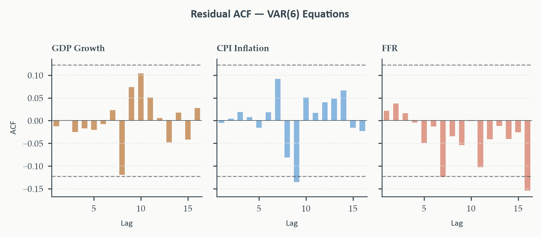
Residual ACF for the VAR(6). The systematic patterns visible in the VAR(1) ACF — the inflation cluster at lags 3–6, the FFR spike at lag 7, the GDP borderline bars — have been substantially reduced. Most bars now fall within the confidence bands. The Durbin-Watson statistics close to 2 confirm that first-order autocorrelation has been removed from all three equations. We proceed with VAR(6) as the working model.

8.4 Granger Causality

Does the Past of One Variable Help Predict Another?

Here is a deceptively simple question: does knowing the history of the federal funds rate help us forecast GDP growth, beyond what GDP growth’s own history already tells us? If the answer is yes — if adding lagged funds rate values to the GDP growth equation reduces forecast errors — then the funds rate Granger-causes GDP growth. If the answer is no — if those lags are collectively redundant — then the funds rate does not Granger-cause GDP growth, in the specific sense that its past carries no marginal predictive content for the growth equation.

Granger causality is a statement about predictive precedence, not about structural or economic causality. Two examples make this clear.

People carry umbrellas before it rains. If we ran a Granger causality test, umbrella-carrying would predict rain: lagged umbrella counts would enter the rain equation with significant coefficients. But umbrellas do not cause rain. Both are driven by a common third factor — forecasted weather — and the umbrella simply comes first in the observable sequence. The Granger test picks up the predictive precedence; it says nothing about the mechanism.

The same logic applies to gift shopping before Christmas. Retail sales surge in November and December, reliably preceding the 25th of December every year. A time series test would find that gift purchases Granger-cause Christmas — but of course the date of Christmas is fixed by the calendar, not by consumer behaviour. The shopping is a leading indicator of a fixed event, not its cause.

Both examples share the same structure: a third variable (weather forecast, the calendar) drives both the leading indicator and the outcome, creating predictive precedence without causal content. In macroeconomics the same problem is pervasive. If financial markets anticipate a recession, asset prices will fall before output does — asset prices will Granger-cause GDP growth, but the true cause may be an underlying shock that markets priced in first. Finding that the funds rate Granger-causes GDP growth does not mean that monetary policy mechanically drives output; it means that past values of the funds rate contain information about future GDP growth that is not already in past values of GDP growth itself. Whether that predictive content reflects a genuine policy transmission or merely the Fed’s response to information that markets had already priced in is a structural question. The direction of a genuine causal mechanism may or may not be recoverable from this reduced-form test — that question belongs to the structural identification of Section 7.5. But as a first-pass description of the predictive relationships in the system, Granger causality is both tractable and informative.

Definition 7.2 — Granger Causality

Variable $x$ Granger-causes variable $y$ if past values of $x$ contain information that helps predict $y$, beyond the information already contained in past values of $y$ alone (and, in a multivariate system, the past values of all other variables in the system). Formally, in the VAR framework:

\[x \not\to_G y \iff \alpha_{ij,\ell} = 0 \quad \text{for all lags } \ell = 1, \ldots, p\]

where $\alpha_{ij,\ell}$ are the coefficients on lags of $x_j$ in the equation for $y_i$. Granger non-causality is the joint hypothesis that the entire block of those coefficients is zero.

The Block Exclusion F-Test

Testing Granger causality in a VAR is an exercise in testing a set of zero restrictions on the coefficient matrices. In the equation for variable $i$, the hypothesis that variable $j$ does not Granger-cause variable $i$ (equation 7.4) is:

\[H_0:\; A_{ij,1} = A_{ij,2} = \cdots = A_{ij,p} = 0 \tag{7.4}\]

This is a system of $p$ linear restrictions on one equation of the VAR. The standard test is the block exclusion F-test: estimate the unrestricted equation (with all $p$ lags of variable $j$ included) and the restricted equation (with those $p$ lags excluded), and compare their residual sums of squares. Under the null, the test statistic follows an $F(p,\, T - np - 1)$ distribution in finite samples, or asymptotically $\chi^2(p)/p$.

In a three-variable VAR, there are $3 \times 2 = 6$ directional Granger causality hypotheses: each variable may or may not Granger-cause each of the other two. We test all six and report them in a single table, which makes the full predictive structure of the system legible at a glance.

Granger Causality Is Not Structural Causality

A finding that $x$ Granger-causes $y$ means that lagged $x$ predicts $y$ in a reduced-form regression. It does not mean that $x$ structurally drives $y$, that the relationship is stable across regimes, or that intervening on $x$ will change $y$. In particular, Granger causality can run from effect to cause if agents anticipate future movements in the causal variable. The federal funds rate may Granger-cause output not because policy drives production but because markets and firms react to anticipated policy changes before they occur. Structural identification — the subject of Section 7.5 — is required to move from predictive precedence to causal interpretation.

Empirical Results

Show code

var_labels = {"GDP Growth": "GDP Growth",
              "CPI Inflation": "CPI Inflation",
              "FFR": "FFR"}

def stars(p):
    if p < 0.01: return "***"
    if p < 0.05: return "** "
    if p < 0.10: return "*  "
    return "   "

# Build list of all directional pairs in readable order
pairs = [(cause, caused)
         for cause in cols
         for caused in cols
         if cause != caused]

header = f"{'Cause':>16}  {'':>4}  {'Effect':>16}  {'p-value':>10}  {'':>4}"
sep    = "─" * len(header)
print(sep)
print(header)
print(sep)

prev_cause = None
for cause, caused in pairs:
    if prev_cause is not None and cause != prev_cause:
        print()          # blank line between cause blocks
    p   = granger_pvals[(cause, caused)]
    sig = stars(p)
    print(f"{cause:>16}  {'→':>4}  {caused:>16}  {p:>10.4f}  {sig:>4}")
    prev_cause = cause

print(sep)
print("H₀: row cause does not Granger-cause column effect.")
print("*** p<0.01  ** p<0.05  * p<0.10")

Table 8.8

──────────────────────────────────────────────────────────
           Cause                  Effect     p-value      
──────────────────────────────────────────────────────────
      GDP Growth     →     CPI Inflation      0.3959      
      GDP Growth     →               FFR      0.0000   ***

   CPI Inflation     →        GDP Growth      0.4592      
   CPI Inflation     →               FFR      0.0488   ** 

             FFR     →        GDP Growth      0.0000   ***
             FFR     →     CPI Inflation      0.0008   ***
──────────────────────────────────────────────────────────
H₀: row cause does not Granger-cause column effect.
*** p<0.01  ** p<0.05  * p<0.10

Granger causality p-values for the three-variable VAR (GDP growth, CPI inflation, FFR), 1954Q3–2019Q4. Each cell reports the p-value for the block exclusion F-test; the null hypothesis is that the row variable does not Granger-cause the column variable.

The results at VAR(6) sharpen the picture relative to the VAR(1) results and reveal a cleaner monetary transmission story. Three relationships are significant at conventional levels.

GDP growth strongly Granger-causes the FFR (p = 0.000): past output growth is a powerful predictor of future rate changes, consistent with the Fed responding to real activity — stronger growth predicts tightening. CPI inflation also Granger-causes the FFR (p = 0.049), confirming the price-stability mandate in the data, though the relationship is weaker than for output. Notably, at VAR(6) inflation’s predictive content for the funds rate is now statistically significant, whereas at VAR(1) it was not (p = 0.739 at the parsimonious model) — the additional lags reveal a delayed inflation-response channel that the parsimonious model missed.

The FFR Granger-causes both GDP growth (p = 0.000) and CPI inflation (p = 0.001). The first confirms the monetary transmission channel: past rate changes contain information about future output that output’s own history cannot supply. The second confirms that policy rate movements predict future inflation — consistent with monetary policy affecting prices with a lag, though the Cholesky IRF will tell us whether this is a disinflationary effect or a price puzzle.

Two relationships are absent. GDP growth does not Granger-cause CPI inflation (p = 0.396), and CPI inflation does not Granger-cause GDP growth (p = 0.459). The first result is the reduced-form Phillips curve non-finding: past output growth has no marginal predictive content for inflation once inflation’s own lags and the other variables are controlled for. This does not contradict the Phillips curve — the contemporaneous and structural relationship between output and prices is better seen in the IRFs — but it does mean the reduced-form feedback runs primarily through the policy rate rather than directly.

What these tests cannot tell us is whether the FFR structurally drives output and inflation — that is the identification question addressed in Section 7.5, where we separate the endogenous policy response from genuine policy shocks.

8.5 SVAR Identification and the Cholesky Decomposition

The Identification Problem

The reduced-form VAR we have estimated so far is useful for forecasting and for Granger causality tests. But its residuals — the vectors $\mathbf{u}_t$ — are not structurally interpretable. Recall from Section 7.1 that these residuals are linear combinations of the underlying structural shocks: $\mathbf{u}_t = \mathbf{A}_0^{-1}\boldsymbol{\varepsilon}_t$, where $\boldsymbol{\varepsilon}_t = [\varepsilon^g_t,\, \varepsilon^\pi_t,\, \varepsilon^r_t]'$ are the genuine independent disturbances to output, inflation, and monetary policy. The reduced-form residual $u^r_t$ in the funds rate equation is not a pure monetary policy shock. It contains a mixture of all three structural shocks, in proportions determined by the unknown elements of $\mathbf{A}_0^{-1}$.

To ask how a monetary policy shock affects GDP growth — the central question of applied monetary economics — we need to disentangle the three structural shocks from the three composite residuals. This requires exactly as many restrictions on $\mathbf{A}_0$ as there are free parameters to recover. With $n = 3$ variables, $\mathbf{A}_0$ has $n^2 = 9$ elements. Normalising the diagonal to ones (so each structural shock has unit contemporaneous effect on its own variable) leaves $n^2 - n = 6$ off-diagonal elements to identify. The covariance matrix of the reduced-form residuals $\boldsymbol{\Sigma}_u = \mathbf{A}_0^{-1}\boldsymbol{\Omega}(\mathbf{A}_0^{-1})'$ — where $\boldsymbol{\Omega}$ is diagonal with structural shock variances — supplies $n(n+1)/2 = 6$ unique equations (the distinct elements of the symmetric matrix). So we have exactly 6 equations and 6 unknowns: the system is just-identified. These equations are nonlinear in the elements of $\mathbf{A}_0$, but the Cholesky restriction — imposing a lower-triangular structure — makes the system triangular, so it can be solved sequentially from the top row down, one element at a time. This is what makes Cholesky identification not just just-identified but analytically tractable.

Cholesky Identification

The most widely used identification scheme imposes a recursive (triangular) structure on $\mathbf{A}_0$. The idea is to order the variables from most exogenous to least exogenous and assume that variable $i$ does not respond contemporaneously to shocks in variables $j > i$ — that is, shocks propagate down the ordering within the period, but not up.

For our system, a natural ordering is: GDP growth first, CPI inflation second, federal funds rate third. The economic rationale is the timing of information within a quarter. Real output and prices are determined by slow-moving production and pricing decisions; the Fed observes these and sets the funds rate in response. Within a single quarter, the assumption is:

A monetary policy shock ($\varepsilon^r_t$) can affect GDP growth and inflation only with a lag — the funds rate is the last to move contemporaneously.
An inflation shock ($\varepsilon^\pi_t$) can affect the funds rate contemporaneously (the Fed reacts to prices within the quarter) but not GDP growth.
An output shock ($\varepsilon^g_t$) can affect both inflation and the funds rate contemporaneously.

This gives $\mathbf{A}_0$ a lower-triangular structure:

\[\mathbf{A}_0 = \begin{bmatrix} 1 & 0 & 0 \\ a_{21} & 1 & 0 \\ a_{31} & a_{32} & 1 \end{bmatrix}\]

The zeros in the upper triangle are the identifying restrictions: inflation does not respond contemporaneously to a monetary policy shock ($a_{12} = 0$), and output responds to neither inflation nor policy within the period ($a_{13} = a_{23} = 0$, or equivalently the first row has no off-diagonal terms in $\mathbf{A}_0^{-1}$).

The Cholesky Decomposition

The Cholesky decomposition of $\boldsymbol{\Sigma}_u$ factors it as $\boldsymbol{\Sigma}_u = \mathbf{P}\mathbf{P}'$ where $\mathbf{P}$ is lower triangular with positive diagonal entries. This is exactly the matrix $\mathbf{A}_0^{-1}\boldsymbol{\Omega}^{1/2}$ implied by the recursive identification. In practice, identification is implemented by applying the Cholesky factor $\mathbf{P}$ to the reduced-form residuals: the orthogonalised shocks $\hat{\boldsymbol{\varepsilon}}_t = \mathbf{P}^{-1}\mathbf{u}_t$ are uncorrelated by construction and have unit variance. These orthogonalised shocks are then used to compute impulse responses and FEVDs.

A Numerical Example

To see where the off-diagonal elements of $\mathbf{P}$ come from, work through the $2 \times 2$ case with variables $g_t$ (GDP growth) and $\pi_t$ (inflation). Suppose the reduced-form residual covariance matrix is:

\[\boldsymbol{\Sigma}_u = \begin{bmatrix} 4.0 & 1.2 \\ 1.2 & 9.0 \end{bmatrix}\]

The diagonal entries are the residual variances ($\sigma^2_{u^g} = 4$, $\sigma^2_{u^\pi} = 9$); the off-diagonal entry is the covariance ($\sigma_{u^g u^\pi} = 1.2$), which is non-zero because the reduced-form residuals mix structural shocks together.

The Cholesky factor $\mathbf{P}$ is lower triangular: $\mathbf{P} = \begin{bmatrix} p_{11} & 0 \\ p_{21} & p_{22} \end{bmatrix}$. The condition $\mathbf{P}\mathbf{P}' = \boldsymbol{\Sigma}_u$ expands to:

\[\begin{bmatrix} p_{11} & 0 \\ p_{21} & p_{22} \end{bmatrix} \begin{bmatrix} p_{11} & p_{21} \\ 0 & p_{22} \end{bmatrix} = \begin{bmatrix} p_{11}^2 & p_{11}p_{21} \\ p_{11}p_{21} & p_{21}^2 + p_{22}^2 \end{bmatrix} = \begin{bmatrix} 4.0 & 1.2 \\ 1.2 & 9.0 \end{bmatrix}\]

The triangular structure makes this sequentially solvable, row by row:

Step 1 — top-left: $p_{11}^2 = 4.0$, so $p_{11} = \sqrt{4.0} = 2.0$. This is the standard deviation of the first structural shock.

Step 2 — off-diagonal: $p_{11}\,p_{21} = 1.2$, so $p_{21} = 1.2 / p_{11} = 1.2 / 2.0 = 0.6$. This is the key step — the off-diagonal element of $\mathbf{P}$ is determined entirely by the covariance between the two reduced-form residuals and the diagonal element already computed. It captures how much of the inflation residual is driven by the output shock (the Cholesky ordering says the output shock can affect inflation contemporaneously, so this cross-loading is permitted).

Step 3 — bottom-right: $p_{21}^2 + p_{22}^2 = 9.0$, so $p_{22} = \sqrt{9.0 - 0.6^2} = \sqrt{8.64} \approx 2.94$. This is the standard deviation of the inflation structural shock — the part of the inflation residual not explained by the output shock.

The result is:

\[\mathbf{P} = \begin{bmatrix} 2.0 & 0 \\ 0.6 & 2.94 \end{bmatrix}\]

The orthogonalised shocks are $\boldsymbol{\varepsilon}_t = \mathbf{P}^{-1}\mathbf{u}_t$. One can verify that $\mathbb{E}[\boldsymbol{\varepsilon}_t\boldsymbol{\varepsilon}_t'] = \mathbf{P}^{-1}\boldsymbol{\Sigma}_u(\mathbf{P}^{-1})' = \mathbf{I}_2$ — the shocks are uncorrelated with unit variance. The three-variable case follows the same sequential logic, adding a third row: solve the diagonal, then the two off-diagonals in order, each depending only on entries already determined above it.

The Ordering Assumption Is Substantive

The Cholesky ordering is not a technical choice — it is an economic one. A different ordering of the same three variables produces different structural shocks and different impulse responses. Reversing the ordering so that the funds rate comes first (as it would if we believed policy was set before output and prices are determined within the quarter) gives a completely different set of orthogonalised shocks. There is no ordering that is obviously correct in all applications, and practitioners routinely check robustness to alternative orderings. The ordering we adopt here — output, inflation, policy rate — is the most common in the monetary policy VAR literature following Christiano, Eichenbaum, and Evans (1999), and its economic rationale is that quarterly GDP and prices are predetermined relative to the policy instrument within the period.

Sign Restrictions as an Alternative

Cholesky identification achieves identification through zero restrictions on the contemporaneous impact matrix — specific variables are assumed not to respond to specific shocks within the period. An alternative approach, increasingly used in modern empirical work, identifies shocks through sign restrictions instead.

Rather than imposing exact zeros, sign restrictions specify only the direction of a shock’s contemporaneous impact. A contractionary monetary policy shock, for example, is defined as one that raises the funds rate, reduces output, and reduces inflation — or at minimum raises the rate and reduces inflation, with output agnostic. Any draw of $\mathbf{A}_0$ consistent with those sign patterns is treated as a valid identification. The set of admissible identifications is typically large, and impulse responses are reported as ranges across that set rather than as point estimates.

Sign restrictions are attractive because they require fewer strong assumptions — exact zeros in $\mathbf{A}_0$ are strong claims — and because they can encode economic theory more directly. A researcher who is confident that a monetary tightening reduces prices but agnostic about timing can say exactly that, without committing to a specific lag structure. The cost is that results are reported as identified sets rather than point estimates, which can be wide when the restrictions are weak. We use Cholesky identification throughout this chapter; sign restrictions are left as a conceptual alternative for projects and further reading.

8.6 Impulse Response Functions

The reduced-form VAR describes how each variable evolves as a linear function of its own past and the past of all other variables. But the object of greatest interest in structural macroeconomics is not the past — it is the future. Specifically: if the economy is hit by an unexpected shock today, how does each variable respond over the next several quarters? This is the question that impulse response functions (IRFs) answer.

A Numerical Example

Before writing down the general formula, it helps to see the recursion produce actual numbers. Start with the simplest possible case: a univariate AR(1), $y_t = \phi y_{t-1} + u_t$. Suppose $\phi = 0.7$ and a unit shock $u_0 = 1$ hits at time $0$. The effect on $y_h$ is:

\[y_0 = 1, \quad y_1 = 0.7, \quad y_2 = 0.49, \quad y_3 = 0.343, \quad \ldots\]

The IRF at horizon $h$ is simply $\phi^h = 0.7^h$. The shock decays geometrically, reaching half its initial size by around $h = 2$ and essentially zero by $h = 10$. This is exactly what the MA($\infty$) representation of an AR(1) says: $y_t = \sum_{h=0}^\infty \phi^h u_{t-h}$, so the coefficient on $u_{t-h}$ is $\phi^h$.

Now extend to a bivariate VAR(1) with variables $g_t$ (GDP growth) and $\pi_t$ (inflation). The values below are illustrative — chosen to keep the arithmetic readable, not estimated from any data — but they are economically plausible: moderate own-persistence, small cross-variable effects, and a Cholesky factor that allows output shocks to have a contemporaneous effect on inflation. Suppose:

\[\mathbf{A}_1 = \begin{bmatrix} 0.6 & 0.2 \\ 0.1 & 0.5 \end{bmatrix}, \qquad \mathbf{P} = \begin{bmatrix} 1.0 & 0 \\ 0.3 & 0.8 \end{bmatrix}\]

where $\mathbf{A}_1$ is the lag-one coefficient matrix and $\mathbf{P}$ is the Cholesky factor. At $h = 0$, the response to a unit output shock ($\varepsilon^g = 1$, $\varepsilon^\pi = 0$) is read directly from the first column of $\mathbf{P}$:

\[\boldsymbol{\Theta}_0 \mathbf{e}_1 = \mathbf{P}\,\mathbf{e}_1 = \begin{bmatrix} 1.0 \\ 0.3 \end{bmatrix}\]

Why the first column? The full matrix $\boldsymbol{\Theta}_0 = \mathbf{P}$ gives the contemporaneous responses to all structural shocks simultaneously — its columns are the $h = 0$ responses to each shock in turn. To isolate the response to shock $j$ only, we apply the unit vector $\mathbf{e}_j$ (all zeros except a 1 in position $j$), giving $_j = $ column $j$ of $\mathbf{P}$. For shock 1 (the output shock), we take column 1. For shock 2 (the inflation shock), we would take column 2, and so on. The diagonal of $\mathbf{P}$ gives only the own-shock own-variable responses — the $h = 0$ values on the main diagonal of the IRF grid — but not the cross-variable contemporaneous impacts. The full column is needed to trace the complete contemporaneous effect of a single shock across all variables.

GDP growth jumps by 1 on impact (the unit normalisation, from $p_{11} = 1$); inflation jumps by 0.3 contemporaneously because $p_{21} = 0.3$ — this is the cross-variable contemporaneous impact permitted by the Cholesky ordering, which allows output shocks to affect inflation within the period. At $h = 1$, the system propagates the impact through $\mathbf{A}_1$:

\[\boldsymbol{\Theta}_1 \mathbf{e}_1 = \mathbf{A}_1 \mathbf{P}\,\mathbf{e}_1 = \begin{bmatrix} 0.6 & 0.2 \\ 0.1 & 0.5 \end{bmatrix} \begin{bmatrix} 1.0 \\ 0.3 \end{bmatrix} = \begin{bmatrix} 0.66 \\ 0.25 \end{bmatrix}\]

At $h = 2$, the response propagates through $\mathbf{A}_1$ again:

\[\boldsymbol{\Theta}_2 \mathbf{e}_1 = \mathbf{A}_1^2 \mathbf{P}\,\mathbf{e}_1 = \begin{bmatrix} 0.6 & 0.2 \\ 0.1 & 0.5 \end{bmatrix} \begin{bmatrix} 0.66 \\ 0.25 \end{bmatrix} = \begin{bmatrix} 0.446 \\ 0.191 \end{bmatrix}\]

The pattern is clear: at each horizon, multiply by $\mathbf{A}_1$ again. In the VAR(1) case, $\boldsymbol{\Theta}_h = \mathbf{A}_1^h \mathbf{P}$, so the IRF is computed by repeatedly powering the coefficient matrix — exactly the multivariate analogue of $\phi^h$ in the scalar case. With $p > 1$ lags, the companion matrix $\mathbf{F}$ plays the role of $\mathbf{A}_1$, as the callout below shows.

From VAR to VMA: The General Formula

The VMA Representation and IRF Formula

For a VAR($p$) written in companion form (equation 7.2) $\boldsymbol{\xi}_t = \mathbf{F}\boldsymbol{\xi}_{t-1} + \tilde{\mathbf{u}}_t$, recursive backward substitution gives the VMA($\infty$) representation:

\[\mathbf{y}_t = \boldsymbol{\mu} + \sum_{h=0}^{\infty} \boldsymbol{\Theta}_h\,\boldsymbol{\varepsilon}_{t-h}\]

where $\boldsymbol{\varepsilon}_t = \mathbf{P}^{-1}\mathbf{u}_t$ are the Cholesky-orthogonalised structural shocks ($\mathbb{E}[\boldsymbol{\varepsilon}_t \boldsymbol{\varepsilon}_t'] = \mathbf{I}_n$) and the orthogonalised IRF matrix at horizon $h$ is:

\[\boldsymbol{\Theta}_h = \mathbf{J}\,\mathbf{F}^h\,\mathbf{J}'\,\mathbf{P}\]

with $\mathbf{J} = [\mathbf{I}_n\;\mathbf{0}\;\cdots\;\mathbf{0}]$ the selection matrix extracting the first $n$ rows of the $np$-dimensional companion system. The $(i,j)$ element $\theta_{ij,h}$ is the impulse response function: the response of variable $i$ to a unit structural shock $j$, $h$ periods after the shock, all other shocks held at zero.

In a stable VAR all eigenvalues of $\mathbf{F}$ lie inside the unit circle, so $\mathbf{F}^h \to \mathbf{0}$ and all IRFs decay to zero — shocks are transitory. The diagonal panels of the IRF grid start at 1.0 by the unit-variance normalisation of $\boldsymbol{\varepsilon}_t$.

Orthogonalisation

The reduced-form shocks $\mathbf{u}_t$ are correlated — $\boldsymbol{\Sigma}_u$ is not diagonal — so a “unit shock to $u^r_t$” is not a well-defined experiment: because $u^g_t$, $u^\pi_t$, and $u^r_t$ move together, hitting one in isolation is not possible. The Cholesky factor $\mathbf{P}$ (Section 7.5) converts them to orthogonal structural shocks $\boldsymbol{\varepsilon}_t = \mathbf{P}^{-1}\mathbf{u}_t$ with $\mathbb{E}[\boldsymbol{\varepsilon}_t\boldsymbol{\varepsilon}_t'] = \mathbf{I}_n$. Substituting into the VMA gives the orthogonalised representation with $\boldsymbol{\Theta}_h = \boldsymbol{\Phi}_h\mathbf{P}$ replacing $\boldsymbol{\Phi}_h$, and it is these orthogonalised matrices that produce structurally interpretable IRFs.

Confidence bands are computed by bootstrapping the VAR residuals: repeatedly redrawing residuals with replacement, re-estimating the VAR and Cholesky factor, recomputing $\boldsymbol{\Theta}_h$ at each draw, and taking the 16th and 84th percentiles of the resulting distribution.

Empirical IRFs

The 3×3 grid of panels is the standard presentation format for a Cholesky-identified VAR with $n$ variables: $n$ columns for the $n$ shocks, $n$ rows for the $n$ response variables, giving $n^2$ panels in total. The layout has a useful built-in diagnostic: the diagonal panels show the response of each variable to its own shock. Because the structural shocks are normalised to unit variance, the contemporaneous own response — the value at horizon $h = 0$ on the diagonal — is always exactly 1 by construction. If you ever see a different value on the diagonal at $h = 0$, the shocks have been scaled differently (for instance, to one standard deviation of the reduced-form residual) or the axes have been re-ordered. The unit diagonal at $h = 0$ is the quickest way to verify that the plot is reading as intended.

Show code

labels       = ["GDP Growth", "CPI Inflation", "FFR"]
colors       = [EO_COPPER, EO_SKYBLUE, EO_TERRACOTTA]
shock_labels = ["Output shock", "Inflation shock", "Policy shock"]
horizons     = np.arange(periods + 1)

fig, axes = plt.subplots(n_vars, n_vars, figsize=(6, 6), sharex=True)

for j in range(n_vars):       # shock (column)
    for i in range(n_vars):   # response (row)
        ax    = axes[i, j]
        color = colors[i]

        point = irf_point[:, i, j]
        lo    = irf_lower[:, i, j]
        hi    = irf_upper[:, i, j]

        ax.fill_between(horizons, lo, hi, color=color, alpha=0.18, lw=0)
        ax.plot(horizons, point, color=color, lw=1.2)
        ax.axhline(0, color=EO_CHARCOAL, lw=0.5, ls="--", alpha=0.5)
        ax.set_xlim(0, periods)
        eo_style_ax(ax)

        if i == 0:
            ax.set_title(shock_labels[j], fontsize=7)
        if j == 0:
            ax.set_ylabel(labels[i], fontsize=7)
        if i == n_vars - 1:
            ax.set_xlabel("Quarters", fontsize=7)

eo_suptitle(fig, "Impulse Response Functions — Three-Variable VAR")
fig.tight_layout()
plt.show()

Figure 8.6: Orthogonalised impulse responses for the three-variable VAR, 1954Q3–2019Q4. Each column corresponds to one structural shock (Cholesky-identified, ordering: GDP growth → CPI inflation → FFR); each row shows the response of one variable. Shaded bands are 16th–84th percentile bootstrap confidence intervals (500 draws). By construction, diagonal panels equal 1 at horizon 0 — each variable’s response to its own unit structural shock. Horizons are in quarters.

Orthogonalised impulse response functions for the three-variable VAR (GDP growth, CPI inflation, federal funds rate), 1954Q3–2019Q4. Cholesky ordering: output → inflation → policy rate. Shaded bands are 16th–84th percentile bootstrap confidence intervals from 500 residual resamples. Diagonal panels start at 1.0 by construction — the unit own-shock normalisation.

The 3×3 layout gives a complete picture of the joint dynamics of the system. Reading across any row traces how a given variable responds to each of the three shocks; reading down any column shows how a given shock propagates across the entire system. The diagonal — own-shock responses — starts at 1.0 in every panel by construction of the unit-variance normalisation, and decays toward zero as the shock dissipates in a stable VAR.

The response of GDP growth to a contractionary policy shock (top-right panel) is the central test of the monetary transmission mechanism. GDP growth falls sharply on impact, reaching a trough of around −1.5 percentage points within the first two quarters before recovering gradually toward zero. The response is clearly negative and precisely estimated — the confidence band stays well below zero for approximately four to five quarters. This is the textbook monetary transmission channel: a surprise tightening depresses real activity with a short but discernible lag, consistent with policy operating through credit conditions, investment, and aggregate demand.

The response of CPI inflation to a policy shock (middle-right panel) shows the price puzzle: inflation rises on impact, peaking around 0.3 percentage points at $h = 1$ before declining slowly toward zero. This is the opposite of the theoretical prediction — a contractionary shock should reduce prices — and is a well-known finding in monetary VARs estimated without commodity prices or other forward-looking inflation indicators. The puzzle arises because our three-variable system cannot fully distinguish a genuine policy shock from an endogenous rate increase in response to anticipated inflation. The VARX result showing that oil prices improve fit (Section 7.8) is directly relevant: adding oil price growth as an exogenous control would likely reduce or eliminate the price puzzle by absorbing the inflationary information the Fed is responding to.

The response of the FFR to an output shock (bottom-left panel) is hump-shaped — the funds rate rises gradually, peaks around $h = 5$ at approximately 0.25 percentage points, then decays back toward zero over the subsequent fifteen quarters. This is the systematic component of monetary policy: the Fed raises rates in response to stronger growth, consistent with the Taylor rule intuition from Section 7.1. The precise timing and magnitude of this response is informative: the peak at $h = 5$ means the Fed tightens roughly five quarters after an output expansion, suggesting a delayed systematic reaction rather than immediate within-quarter adjustment.

8.7 Forecast Error Variance Decomposition

How Much of the Variance Comes From Each Shock?

The impulse response function answers a path question: given a shock today, how does each variable move over the next $h$ periods? The forecast error variance decomposition (FEVD) answers an attribution question: of all the uncertainty in our $h$-step-ahead forecast of variable $i$, what fraction is due to each structural shock?

To see why this question is non-trivial, consider what happens after a single policy shock — a surprise increase in the federal funds rate. At $h = 0$ the shock hits the funds rate equation directly. But through the VAR’s coefficient matrices it then propagates forward: higher rates dampen GDP growth over the next several quarters; weaker growth in turn reduces inflationary pressure; lower inflation feeds back into the funds rate as the Fed responds. By $h = 8$, a shock that originated entirely in the policy equation has generated forecast errors in all three variables — not because multiple shocks occurred, but because a single shock rippled through the system.

If we imagine hitting the economy with all three structural shocks simultaneously — output, inflation, and policy shocks all firing at once — the total forecast uncertainty in GDP growth at horizon $h$ is the sum of their individual contributions. The FEVD asks: what share of that total comes from each source? A policy shock that ripples strongly into GDP growth will claim a large share of GDP growth’s forecast variance at horizons where its IRF is large. An inflation shock whose effect on GDP growth is small and short-lived will claim a small share. The FEVD translates the IRF paths into a single percentage at each horizon: the fraction of forecast uncertainty attributable to each structural disturbance.

Deriving the Decomposition

The $h$-step-ahead forecast error for variable $i$ is the cumulative effect of all structural shocks that occur between the forecast origin and the target period. From the VMA representation derived in Section 7.6:

\[y_{i,t+h} - \hat{y}_{i,t+h|t} = \sum_{s=0}^{h-1} \sum_{j=1}^{n} \theta_{ij,s}\,\varepsilon_{j,t+h-s} \tag{7.5}\]

The forecast error variance of variable $i$ at horizon $h$ is therefore:

\[\text{MSE}_{i}(h) = \sum_{s=0}^{h-1} \sum_{j=1}^{n} \theta_{ij,s}^2 = \sum_{j=1}^{n} \underbrace{\sum_{s=0}^{h-1} \theta_{ij,s}^2}_{\text{contribution of shock } j} \tag{7.6}\]

where the second equality uses the fact that structural shocks are orthogonal ($\mathbb{E}[\varepsilon_{j,t}\varepsilon_{k,t}] = 0$ for $j \neq k$) so cross-terms vanish. The FEVD share of shock $j$ in the variance of variable $i$ at horizon $h$ is:

\[\omega_{ij}(h) = \frac{\displaystyle\sum_{s=0}^{h-1} \theta_{ij,s}^2} {\displaystyle\sum_{k=1}^{n}\sum_{s=0}^{h-1} \theta_{ik,s}^2} \tag{7.7}\]

By construction $\sum_{j=1}^{n} \omega_{ij}(h) = 1$ at every horizon: the shares sum to 100 percent (equations 7.5–7.7). At $h = 1$, the FEVD equals the contemporaneous impact of each shock — only the $h=0$ IRF coefficient matters, so the decomposition reflects the Cholesky ordering directly. At longer horizons, the cumulative squared IRF paths determine the shares, and the ordering assumption becomes less influential as later-horizon dynamics dominate.

Definition 7.3 — Forecast Error Variance Decomposition

The FEVD share $\omega_{ij}(h)$ is the fraction of the $h$-step forecast error variance of variable $i$ that is attributable to structural shock $j$:

\[\omega_{ij}(h) = \frac{\sum_{s=0}^{h-1} \theta_{ij,s}^2} {\sum_{k=1}^{n}\sum_{s=0}^{h-1} \theta_{ik,s}^2}, \qquad \sum_{j=1}^{n}\omega_{ij}(h) = 1\]

The shares are horizon-dependent: a shock that dominates at short horizons may be less important at long horizons if other shocks have slower-building but more persistent effects.

Empirical FEVD

Show code

labels      = ["GDP Growth", "CPI Inflation", "FFR"]
shock_names = ["Output", "Inflation", "Policy"]
horizons_tbl = [1, 4, 8, 12, 20]

col_w  = 12
h_w    = 6

for i, var_label in enumerate(labels):
    header = (f"\n{'':>{h_w}}" +
              "".join(f"{s:>{col_w}}" for s in shock_names))
    sep    = "─" * (h_w + col_w * len(shock_names))
    print(f"Dependent variable: {var_label}")
    print(sep)
    print(header)
    print(sep)
    for h in horizons_tbl:
        row = f"{'h='+str(h):>{h_w}}"
        for j in range(len(shock_names)):
            share = fevd_decomp[i, h - 1, j] * 100
            row  += f"{share:>{col_w}.1f}"
        print(row)
    print(sep)
    print("Shares in percent; rows sum to 100.")

Table 8.9

Dependent variable: GDP Growth
──────────────────────────────────────────

            Output   Inflation      Policy
──────────────────────────────────────────
   h=1       100.0         0.0         0.0
   h=4        92.1         0.6         7.3
   h=8        88.8         2.1         9.1
  h=12        87.5         3.4         9.1
  h=20        87.2         3.6         9.2
──────────────────────────────────────────
Shares in percent; rows sum to 100.
Dependent variable: CPI Inflation
──────────────────────────────────────────

            Output   Inflation      Policy
──────────────────────────────────────────
   h=1         0.0       100.0         0.0
   h=4         2.0        91.5         6.5
   h=8         6.4        86.2         7.3
  h=12         8.3        84.5         7.2
  h=20         9.3        83.7         7.1
──────────────────────────────────────────
Shares in percent; rows sum to 100.
Dependent variable: FFR
──────────────────────────────────────────

            Output   Inflation      Policy
──────────────────────────────────────────
   h=1         6.5         3.0        90.5
   h=4        36.3         6.9        56.8
   h=8        49.1        14.8        36.1
  h=12        51.7        20.2        28.1
  h=20        51.2        24.8        24.0
──────────────────────────────────────────
Shares in percent; rows sum to 100.

Forecast error variance decompositions for the three-variable VAR (GDP growth, CPI inflation, FFR), 1954Q3–2019Q4. Shares in percent; rows sum to 100. Cholesky ordering: output → inflation → policy rate.

Show code

var_labels  = ["GDP Growth", "CPI Inflation", "FFR"]
shock_names = ["Output shock", "Inflation shock", "Policy shock"]
colors      = [EO_COPPER, EO_SKYBLUE, EO_TERRACOTTA]
horizons_p  = np.arange(1, periods + 1)

fig, axes = plt.subplots(1, 3, figsize=(6, 3), sharey=True)

for i, (ax, var_label) in enumerate(zip(axes, var_labels)):
    # shares: shape (periods, n_shocks) — fevd_decomp[i, h, j]
    shares = np.array([fevd_decomp[i, h, :] * 100
                       for h in range(periods)])   # (periods, n)

    bottom = np.zeros(periods)
    for j, (shock_name, color) in enumerate(zip(shock_names, colors)):
        ax.fill_between(horizons_p, bottom, bottom + shares[:, j],
                        color=color, alpha=0.75, lw=0,
                        label=shock_name if i == 0 else None)
        bottom += shares[:, j]

    ax.set_xlim(1, periods)
    ax.set_ylim(0, 100)
    ax.set_xlabel("Quarters", fontsize=7)
    ax.set_title(var_label, fontsize=8)
    eo_style_ax(ax)

axes[0].set_ylabel("Share of forecast variance (%)", fontsize=7)
fig.legend(loc="lower center", ncol=3, fontsize=6,
           bbox_to_anchor=(0.5, -0.12), frameon=True)
eo_suptitle(fig, "Forecast Error Variance Decomposition")
fig.tight_layout()
plt.show()

Figure 8.7: Forecast error variance decompositions for the three-variable VAR, 1954Q3–2019Q4. Each panel shows the fraction of forecast error variance in one variable attributable to each structural shock (Cholesky ordering: output → inflation → policy rate) as the horizon grows from 1 to 20 quarters. Stacked areas sum to 100 percent at every horizon.

Stacked area FEVD for the three-variable VAR(6). GDP growth variance (left) is dominated by the output shock throughout, but the policy shock (terracotta) claims a visible 7–9 percent share from $h = 4$ onward — larger than at VAR(1). CPI inflation variance (centre) is dominated by the own-shock (sky blue) at all horizons, with output and policy shocks making only modest inroads by $h = 20$. FFR variance (right) shows the most dramatic redistribution: the policy own-shock (terracotta) falls from 91 percent at $h = 1$ to 24 percent at $h = 20$ as the output shock (copper) rises to 51 percent — quantifying the Fed’s systematic response to real conditions.

The results tell a consistent story across all three variables, and differ meaningfully from the VAR(1) estimates — illustrating why model selection and diagnostic checking matter before structural analysis.

GDP growth remains predominantly self-driven but the policy shock now claims a meaningful share at medium horizons. The output shock accounts for 100 percent at $h = 1$ by Cholesky construction, falls to 92 percent by $h = 4$, and stabilises around 87 percent at $h = 20$. Policy shocks account for 7–9 percent of GDP growth variance from $h = 4$ onward — small in absolute terms but larger than the 1–2 percent seen in the VAR(1) estimates. The message is nuanced: autonomous output shocks dominate business cycle fluctuations, but the unexpected component of monetary policy accounts for a non-trivial share of medium-run output variance. This is consistent with the IRF finding that policy shocks produce a sharp GDP growth contraction of around 1.5 percentage points.

CPI inflation is dominated by its own shocks throughout, but the pattern differs strikingly from GDP growth. At $h = 1$ inflation is entirely self-driven by Cholesky construction (100 percent own-shock). By $h = 4$ the own-shock share is still 92 percent, but by $h = 20$ it has declined to 84 percent, with output shocks accounting for 9 percent and policy shocks for 7 percent. The relatively modest policy share — despite the Granger causality finding that the FFR predicts inflation — is consistent with the price puzzle in the IRF: what the Granger test picks up as “FFR predicts inflation” is partly the Fed raising rates in anticipation of inflation that then materialises, not a structural disinflationary effect. The persistent dominance of own-shock reflects genuine autonomous inflation dynamics — supply shocks, expectation shifts — that are not driven by either output or monetary policy within this sample.

FFR variance shows the most dramatic horizon redistribution in the system. At $h = 1$, 91 percent of policy rate variance comes from policy shocks — the Fed is making largely discretionary decisions. But by $h = 4$ the output shock share has surged to 36 percent, and by $h = 12$ it reaches 52 percent, where it stabilises. The inflation shock share grows more slowly, reaching 25 percent by $h = 20$. By the twenty-quarter horizon, only 24 percent of FFR variance is attributable to autonomous policy innovations — the majority reflects the endogenous response to real and nominal conditions. This is a strong quantitative statement of the Fed’s systematic behaviour: at business cycle frequencies, most interest rate variation is predictable from output and inflation dynamics, not from discretionary surprises.

8.8 Adding Exogenous Variables: The VARX

The VAR treats every variable in the system symmetrically — each one has its own equation, its own structural shock, and contributes to the FEVD of every other variable. This is the right framework when we believe all variables are jointly determined and we want to understand how shocks propagate among them. But sometimes we want to condition on a variable without modelling it. There are at least three situations where this arises.

First, the variable may be genuinely exogenous to the system — determined outside the domestic economy and therefore unaffected by shocks to any of the endogenous variables. Oil prices are the canonical example in macro VARs: US output and inflation cannot plausibly move world crude prices, so treating oil as endogenous would model a feedback channel that does not exist, waste degrees of freedom, and potentially distort the identified shocks.

Second, we may simply not care about the variable’s dynamics. A researcher studying monetary transmission wants to know how a policy shock affects output and inflation — not what drives oil prices. Adding oil as an exogenous control absorbs its influence on the endogenous variables without requiring a model for the oil market itself.

Third, the variable may be a policy instrument or external shock that is best treated as a conditioning variable for identification purposes — commodity prices as an inflation predictor, foreign interest rates as a transmission channel, or a fiscal policy index as a control for budget conditions.

The ARMAX model in Chapter 3 handled this case for a single equation. The multivariate extension is the VARX, which appends a matrix of exogenous regressors to the reduced-form VAR.

The VARX($p$, $s$) Model

Let $\mathbf{x}_t$ be a $k \times 1$ vector of exogenous variables. The VARX($p$, $s$) model is:

\[\mathbf{y}_t = \mathbf{c} + \sum_{\ell=1}^{p}\mathbf{A}_\ell\,\mathbf{y}_{t-\ell} + \sum_{j=0}^{s}\mathbf{B}_j\,\mathbf{x}_{t-j} + \mathbf{u}_t \tag{7.8}\]

where $\mathbf{B}_j$ is an $n \times k$ matrix of coefficients on the $j$-th lag of the exogenous block. The lag order $s$ governs how many lags of $\mathbf{x}_t$ enter each equation; $s = 0$ means only contemporaneous values, $s = 1$ adds one lag, and so on. Each equation receives the same exogenous regressors — this is what distinguishes the VARX from a set of unrelated ARMAX equations. The endogenous block $\mathbf{u}_t$ retains its interpretation as before: correlated reduced-form innovations that mix the structural shocks together.

Estimation is still OLS equation by equation, with the exogenous regressors treated as fixed regressors in each equation. Lag selection for $p$ and $s$ proceeds jointly using AIC or BIC, with the penalty now covering both the $n^2 p$ endogenous slope coefficients and the $nk(s+1)$ exogenous coefficients (equation 7.8).

What Changes — and What Does Not

Changes: The coefficient matrices $\mathbf{B}_j$ absorb the linear effect of $\mathbf{x}_t$ on each endogenous variable. IRFs and FEVDs for the endogenous block are computed exactly as in the pure VAR, but the baseline forecasts are shifted by the exogenous variables’ paths. Scenario analysis — asking how the endogenous variables would respond under a specific path for $\mathbf{x}_t$ — is straightforward: feed the assumed $\mathbf{x}_t$ path into the forecast equations.

Does not change: The exogenous variables do not receive structural shocks in the SVAR sense. They do not appear in the FEVD of the endogenous variables (unless the FEVD is explicitly extended to include exogenous contributions, which requires additional modelling assumptions). The identification problem for the endogenous block is unchanged: the Cholesky ordering applies only to $\boldsymbol{\Sigma}_u$, not to $\mathbf{x}_t$.

Why Lagged Exogenous Variables Matter in a VARX but Not in an ARMAX

It is worth asking why the VARX includes $s$ lags of $\mathbf{x}_t$ rather than just the contemporaneous value. In a single-equation ARMAX, the argument for omitting lagged $x_t$ is compelling: if $x_t$ is serially correlated, its past values are correlated with past values of $y_t$, which are already captured by the AR lags. Adding $x_{t-1}$ explicitly provides little marginal information beyond what the AR component already absorbs.

The VARX case is different for two reasons.

First, $\mathbf{x}_t$ is by assumption outside the endogenous system — that is the entire motivation for treating it as exogenous. If oil prices have dynamics that are partly orthogonal to domestic output, inflation, and the funds rate, then past values of $\mathbf{y}_t$ do not fully reconstruct past values of $\mathbf{x}_t$. The information in $\mathbf{x}_{t-1}$ is genuinely not redundant given $\mathbf{y}_{t-1}, \mathbf{y}_{t-2}, \ldots$

Second, the transmission from $\mathbf{x}_t$ to $\mathbf{y}_t$ may be delayed. An oil price shock in quarter $t$ may affect GDP growth in quarter $t+1$ through investment and spending decisions that take time to adjust. In the ARMAX, the AR lags pick up this delayed effect indirectly — the contemporaneous impact of $x_t$ on $y_t$ creates a correlation between $y_{t+1}$ and $x_t$ that the AR component absorbs. In the VARX, where $\mathbf{x}_t$ is orthogonal to $\mathbf{u}_t$ by assumption, the only way to capture a delayed effect of $\mathbf{x}_{t-1}$ on $\mathbf{y}_t$ is to include $\mathbf{x}_{t-1}$ explicitly.

The clean summary: in an ARMAX the AR component and $x_t$ share the same dependent variable, so lagged $x_t$ is indeed largely redundant given enough AR lags. In a VARX, $\mathbf{x}_t$ lives outside the endogenous system and its lags carry information that the endogenous lags cannot reconstruct. The practical implication is that $s$ should be chosen by information criteria alongside $p$, rather than set to zero by default.

Stationarity of Exogenous Variables

The stationarity requirement for endogenous variables is clear: all $\mathbf{y}_t$ must be $I(0)$. For exogenous variables the answer is more nuanced, and getting it wrong has the same consequences as including $I(1)$ variables in levels in a pure VAR.

Stationarity Rules for Exogenous Variables

$\mathbf{x}_t$ is $I(0)$: include in levels. No adjustment needed.
$\mathbf{x}_t$ is $I(1)$, not cointegrated with $\mathbf{y}_t$: include in first differences. Including the level would introduce a stochastic trend into each equation’s error term, producing spurious coefficient estimates for the same reason as a static regression of $I(1)$ on $I(1)$ variables.
$\mathbf{x}_t$ is $I(1)$, cointegrated with $\mathbf{y}_t$: the correct framework is a VECMX — a vector error correction model with exogenous variables — which includes the cointegrating residual as an error correction term. This is Chapter 8 territory. The practical rule: if you suspect cointegration between an exogenous and an endogenous variable, treat the exogenous variable as endogenous and use the VECM framework.

When in doubt, first-difference the $I(1)$ exogenous variable. The cost of over-differencing (losing level information) is smaller than the cost of spurious regression.

Empirical Example: Oil Prices as an Exogenous Variable

Oil price shocks are one of the most studied external drivers of US macroeconomic fluctuations. The 1973 OPEC embargo, the 1979 Iranian Revolution, and the 2007–08 price surge all coincided with US recessions, suggesting that oil prices carry information about future output and inflation beyond what the domestic VAR already captures. We add the annualised quarterly growth rate of WTI crude oil prices as an exogenous variable — $\Delta \ln(\text{oil}_t) \times 400$ — to our three-variable VAR.

Oil price growth is $I(0)$ (oil prices in levels are $I(1)$, but their log growth rate is stationary), so no transformation beyond the log-differencing is required. We include contemporaneous oil price growth only ($s = 0$) as a first pass, consistent with the interpretation that oil prices affect the domestic economy within the quarter.

Show code

print(f"ADF test — WTI oil price growth (annualised %, quarterly)")
print(f"  Statistic : {oil_adf[0]:.3f}")
print(f"  p-value   : {oil_adf[1]:.4f}")
print(f"  Crit (5%) : {oil_adf[4]['5%']:.3f}")
print(f"  Decision  : {'Stationary — include in levels' if oil_adf[1] < 0.05 else 'Unit root?'}")

Table 8.10

ADF test — WTI oil price growth (annualised %, quarterly)
  Statistic : -11.567
  p-value   : 0.0000
  Crit (5%) : -2.873
  Decision  : Stationary — include in levels

ADF pre-check for WTI oil price growth, the exogenous variable added to the VARX. The test statistic of −11.567 (p = 0.000) rejects the unit root null decisively — oil price growth is stationary and suitable for direct inclusion as a contemporaneous exogenous regressor without further transformation.

Show code

print("Model comparison: VAR vs VARX (oil price growth as exogenous)")
print()
header = f"{'Model':<20}  {'BIC':>12}  {'ΔBIC':>10}"
sep    = "─" * len(header)
print(sep)
print(header)
print(sep)
print(f"{'VAR(' + str(p_final) + ')':<20}  {var_bic:>12.3f}  {'—':>10}")
delta = varx_bic - var_bic
better = "VARX preferred" if delta < 0 else "VAR preferred"
print(f"{'VARX(' + str(p_final) + ',0)':<20}  {varx_bic:>12.3f}  {delta:>10.3f}")
print(sep)
print(f"Δ BIC = VARX − VAR. Negative favours VARX. {better}.")
print("Note: BIC reported per observation by statsmodels.")

Table 8.11

Model comparison: VAR vs VARX (oil price growth as exogenous)

──────────────────────────────────────────────
Model                          BIC        ΔBIC
──────────────────────────────────────────────
VAR(6)                       2.406           —
VARX(6,0)                    2.226      -0.180
──────────────────────────────────────────────
Δ BIC = VARX − VAR. Negative favours VARX. VARX preferred.
Note: BIC reported per observation by statsmodels.

BIC comparison between the pure VAR(6) and the VARX(6,0) with contemporaneous oil price growth, 1954Q3–2019Q4. The VARX has a lower BIC (2.226 vs 2.406, $\Delta = -0.180$), indicating that adding contemporaneous oil price growth improves fit enough to more than compensate for the additional three parameters (one per equation). The VARX is preferred.

The BIC result is economically interpretable. The VARX’s lower BIC confirms that domestic output, inflation, and the funds rate have a systematic contemporaneous relationship with oil price movements that six lags of the endogenous variables alone cannot capture — consistent with the supply-shock narrative. Oil price surprises shift the inflation equation directly within the quarter, compress output, and trigger a policy response, all in ways that are orthogonal to the VAR’s own dynamics. Conditioning on oil price growth therefore tightens the VAR residuals and improves the identification of the domestic monetary policy shock.

For applications involving series plausibly affected by external drivers — commodity prices, trade volumes, foreign interest rates — the VARX offers a principled way to condition on those drivers without modelling them. The workflow is: test the exogenous variable for stationarity, transform if necessary, pass it as the exog argument to statsmodels VAR, and compare information criteria against the pure VAR to assess whether inclusion is warranted. When the VARX is preferred, re-running the Granger causality tests and IRF analysis on the VARX is recommended: the structural shocks will be better identified once the exogenous information is absorbed into the residuals, and results that appeared significant — or insignificant — in the pure VAR may change once the external driver is properly controlled for.

8.9 When Variables Are I(1)

Everything in this chapter has assumed that all three variables in the VAR are stationary. The ADF tests in Section 7.2 confirmed this cleanly for GDP growth and CPI inflation; for the FFR the ADF did not reject, but the lag polynomial roots in Table 7.2 confirmed that the estimated VAR is stable — the definitive check. Many applications are less fortunate: price levels, nominal GDP, exchange rates, and interest rates over very long samples can exhibit behaviour consistent with genuine unit roots that survive both tests.

If we attempt to estimate a VAR in levels with $I(1)$ variables, we face the same problem identified in Chapter 4 for univariate regressions. OLS coefficient estimates are still consistent — the VAR is at least not spurious in the same way as a static regression — but the standard distributions for $t$-statistics, $F$-statistics, and information criteria no longer apply. Lag selection by AIC or BIC is unreliable. Granger causality F-tests have non-standard distributions under the null. Impulse responses computed from a VAR in $I(1)$ levels do not converge to zero as $h \to \infty$ — they approach a non-zero constant, reflecting the permanent effects of shocks in an integrated system. The unit-eigenvalue structure of the companion matrix that stationarity rules out is present by construction.

The naive fix is to difference every $I(1)$ variable before including it in the VAR. A VAR in first differences — $\Delta \mathbf{y}_t$ — restores stationarity and makes all the tools of this chapter valid. But differencing has a cost: it removes all information about long-run levels. If GDP and consumption share a common stochastic trend — if they are cointegrated — a VAR in differences cannot capture that relationship. The error correction mechanism, which describes how deviations from the long-run relationship are corrected over time, is invisible to a differenced VAR.

Cointegration and the Path to Chapter 8

Two $I(1)$ series are cointegrated if there exists a linear combination of them that is $I(0)$ — stationary. The classic example is consumption and income: neither is stationary in levels, but the ratio of consumption to income (or equivalently, their log difference) fluctuates around a stable mean. A VAR in differences applied to cointegrated series is misspecified — it omits the error correction term that describes the long-run equilibrium, and its forecasts and IRFs are therefore distorted at long horizons.

The correct model for a system of cointegrated $I(1)$ variables is the vector error correction model (VECM). The VECM rewrites the VAR in a way that explicitly separates the short-run dynamics (changes in each variable, the differenced part) from the long-run equilibrium relationship (the cointegrating vector, the levels part). It nests the VAR in differences as a special case — when there is no cointegration — and adds the error correction terms that describe how the system returns to its long-run attractor after a shock.

Do Not Estimate a VAR in Levels with I(1) Variables

If unit root tests suggest that one or more variables in your system are $I(1)$, estimating a VAR in levels produces unreliable inference. The correct path is:

Test each variable for unit roots (Chapter 4 tools).
Test for cointegration among the $I(1)$ variables (Johansen test — Chapter 8).
If cointegration is found, estimate a VECM.
If no cointegration is found, estimate a VAR in first differences.

A VAR in levels with $I(1)$ variables is neither of these. Do not use it.

8.10 Looking Ahead

This chapter built the complete reduced-form and structural VAR toolkit: from the endogeneity motivation through lag selection, Granger causality, Cholesky identification, impulse responses, and variance decomposition. The tools are powerful, but they rest on a maintained assumption that every variable in the system is stationary. Section 7.9 showed what happens when that assumption fails and pointed toward two responses: difference the variables, or model the long-run relationship explicitly. The first option discards information about long-run relationships between variables; the second requires a framework that does not yet exist in our toolkit.

Chapter 8 — Cointegration and the Vector Error Correction Model develops that framework. When two or more $I(1)$ variables share a common stochastic trend — when they are cointegrated — the vector error correction model (VECM) provides a complete description of their joint dynamics. The VECM reparameterises the VAR in levels so that short-run dynamics and the long-run equilibrium relationship appear as distinct, estimable components. Determining how many long-run relationships exist requires the Johansen trace test, a procedure that examines the rank of the long-run coefficient matrix $\boldsymbol{\Pi}$ through its eigenvalues: a rank of zero means no cointegration and a VAR in first differences is appropriate; a positive rank means the variables share common stochastic trends and the VECM is required.

The running example will be the US yield curve — the 10-year Treasury yield and the 3-month T-bill rate. The expectations hypothesis of the term structure predicts that these two rates are cointegrated with a cointegrating vector of $(1, -1)'$: both rates are driven by the same monetary policy and inflation expectations, so their spread should be stationary around a constant term premium rather than drifting. That spread is also one of the most reliable recession indicators in macroeconomics — yield curve inversions have preceded every US recession since 1954 — and the VECM gives us a precise language for understanding why: an inversion is an extreme deviation from the long-run equilibrium, and the error correction mechanism predicts the forces that eventually restore a positive spread.

8.11 Key Terms

Glossary

Vector autoregression VAR($p$) — A system of $n$ equations in which each variable is modelled as a linear function of $p$ lags of all variables in the system plus a composite innovation: $\mathbf{y}_t = \mathbf{c} + \sum_{\ell=1}^{p}\mathbf{A}_\ell\mathbf{y}_{t-\ell} + \mathbf{u}_t$. The reduced form is estimable by OLS equation by equation; its coefficients are not structurally interpretable without additional identifying restrictions.

Companion matrix $\mathbf{F}$ — The $np \times np$ matrix that writes any VAR($p$) as a first-order system $\boldsymbol{\xi}_t = \mathbf{F}\boldsymbol{\xi}_{t-1} + \tilde{\mathbf{u}}_t$. Its eigenvalues are the $np$ characteristic roots of the VAR. Stability requires all eigenvalues inside the unit circle. Also used to compute IRFs via $\boldsymbol{\Theta}_h = \mathbf{J}\mathbf{F}^h\mathbf{J}'\mathbf{P}$.

Granger causality — Variable $x$ Granger-causes variable $y$ if past values of $x$ have marginal predictive content for $y$ beyond the information in past values of $y$ (and all other variables in the system). Tested by the block exclusion F-test: $H_0$ is that all $p$ coefficients on lags of $x$ in the $y$ equation are jointly zero. A statement about predictive precedence, not structural causality.

Structural VAR (SVAR) — A VAR augmented with identifying restrictions on the contemporaneous impact matrix $\mathbf{A}_0$ that allow the reduced-form composite residuals $\mathbf{u}_t = \mathbf{A}_0^{-1}\boldsymbol{\varepsilon}_t$ to be decomposed into interpretable structural shocks $\boldsymbol{\varepsilon}_t$. With $n$ variables, just-identification requires $n(n-1)/2$ restrictions beyond the $n$ diagonal normalisations.

Cholesky identification — A recursive identifying scheme that imposes a lower-triangular structure on $\mathbf{A}_0$, equivalent to factoring $\boldsymbol{\Sigma}_u = \mathbf{P}\mathbf{P}'$ and defining orthogonalised shocks as $\boldsymbol{\varepsilon}_t = \mathbf{P}^{-1}\mathbf{u}_t$. The ordering of variables determines which contemporaneous effects are set to zero; the ordering is an economic assumption, not a statistical one.

Impulse response function (IRF) — $\text{IRF}_{ij}(h) = \theta_{ij,h}$, the response of variable $i$ to a unit structural shock $j$ at horizon $h$, computed as the $(i,j)$ element of $\boldsymbol{\Theta}_h = \mathbf{J}\mathbf{F}^h\mathbf{J}'\mathbf{P}$. In a stable VAR all IRFs converge to zero. Presented as the $n \times n$ grid of panels, with diagonal own-shock responses starting at 1 by the unit-variance normalisation.

Forecast error variance decomposition (FEVD) — The share $\omega_{ij}(h)$ of the $h$-step forecast error variance of variable $i$ attributable to structural shock $j$: $\omega_{ij}(h) = \sum_{s=0}^{h-1}\theta_{ij,s}^2 \,/\, \sum_{k}\sum_{s=0}^{h-1}\theta_{ik,s}^2$. Shares sum to 100 percent at every horizon. Horizon-dependent: short-run and long-run attributions can differ substantially.

Price puzzle — The empirical finding in some estimated monetary VARs that a contractionary policy shock is followed by a rise in inflation, contradicting theory. Typically attributed to imperfect identification: the funds rate increase is partly an endogenous response to anticipated inflation not yet visible in the CPI, so the estimated IRF conflates the policy action with the inflationary pressure it was responding to.

Sign restrictions — An identification scheme that recovers structural shocks by restricting the sign of their contemporaneous or short-run impacts rather than setting specific elements to zero. A contractionary policy shock is defined as one that raises the funds rate and reduces inflation; any $\mathbf{A}_0$ consistent with those sign patterns is admissible. Results are reported as identified sets (ranges of IRFs) rather than point estimates.

VARX($p$, $s$) — A VAR($p$) augmented with $s + 1$ lags of a $k \times 1$ vector of exogenous variables $\mathbf{x}_t$: $\mathbf{y}_t = \mathbf{c} + \sum_\ell \mathbf{A}_\ell \mathbf{y}_{t-\ell} + \sum_j \mathbf{B}_j \mathbf{x}_{t-j} + \mathbf{u}_t$. Exogenous variables are conditioned on but not modelled; they do not receive structural shocks and do not enter the FEVD of the endogenous block. Exogenous variables must be $I(0)$; $I(1)$ exogenous variables should be first-differenced before inclusion unless cointegration with the endogenous block is modelled explicitly via a VECMX.

Cointegration — Two or more $I(1)$ series are cointegrated if a linear combination of them is $I(0)$. Cointegrated series share a common stochastic trend and cannot drift arbitrarily far apart. A VAR in first differences applied to cointegrated series is misspecified — it omits the error correction mechanism that describes the long-run equilibrium. The appropriate model is the VECM, developed in Chapter 8 following the Johansen test for cointegrating rank.

Vector error correction model (VECM) — A reparameterisation of a VAR for cointegrated $I(1)$ variables that separates short-run dynamics (in first differences) from the long-run equilibrium relationship (the cointegrating vector, which acts as an error correction term pulling the system back toward equilibrium after shocks). The VECM is a special case of a state space model: the cointegrating residual is an unobserved state estimated optimally by the Kalman filter. Full treatment in Chapter 11.

8.1 Why Univariate Models Are Not Enough

A Structural System and Its Reduced Form

Extending to Three Variables

8.2 The Reduced-Form VAR

From Two Variables to \(n\)

The Stationarity Condition

8.3 VAR Estimation and Model Selection

Why Lag Length Matters More in a VAR

Information Criteria for VARs

The Likelihood Ratio Test

Lag Selection Results

Estimated VAR(1)

Stability: VAR(1)

Residual Diagnostics: VAR(1)

From VAR(1) to VAR(6): How a Researcher Proceeds

The Working Model: VAR(6)

Residual Diagnostics: VAR(6)

8.4 Granger Causality

Does the Past of One Variable Help Predict Another?

The Block Exclusion F-Test

Empirical Results

8.5 SVAR Identification and the Cholesky Decomposition

The Identification Problem

Cholesky Identification

A Numerical Example

Sign Restrictions as an Alternative

8.6 Impulse Response Functions

A Numerical Example

From VAR to VMA: The General Formula

Orthogonalisation

Empirical IRFs

8.7 Forecast Error Variance Decomposition

How Much of the Variance Comes From Each Shock?

Deriving the Decomposition

Empirical FEVD

8.8 Adding Exogenous Variables: The VARX

The VARX(\(p\), \(s\)) Model

Why Lagged Exogenous Variables Matter in a VARX but Not in an ARMAX

Stationarity of Exogenous Variables

Empirical Example: Oil Prices as an Exogenous Variable

8.9 When Variables Are I(1)

Cointegration and the Path to Chapter 8

8.10 Looking Ahead

8.11 Key Terms