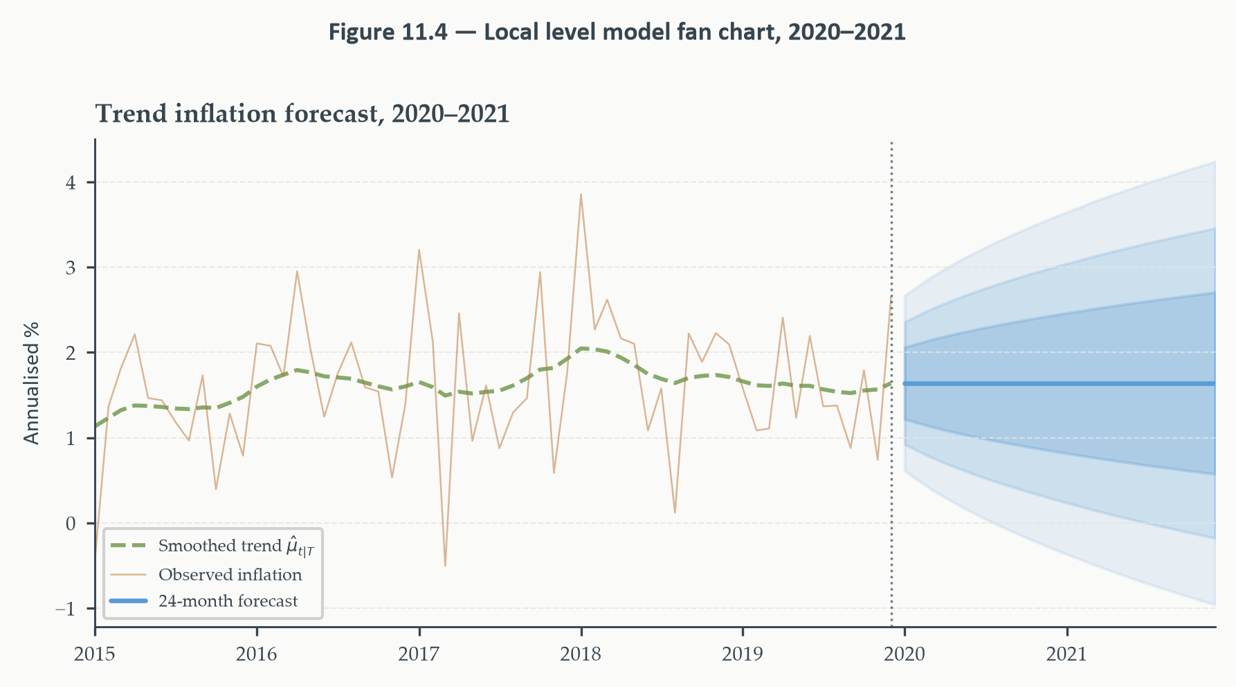
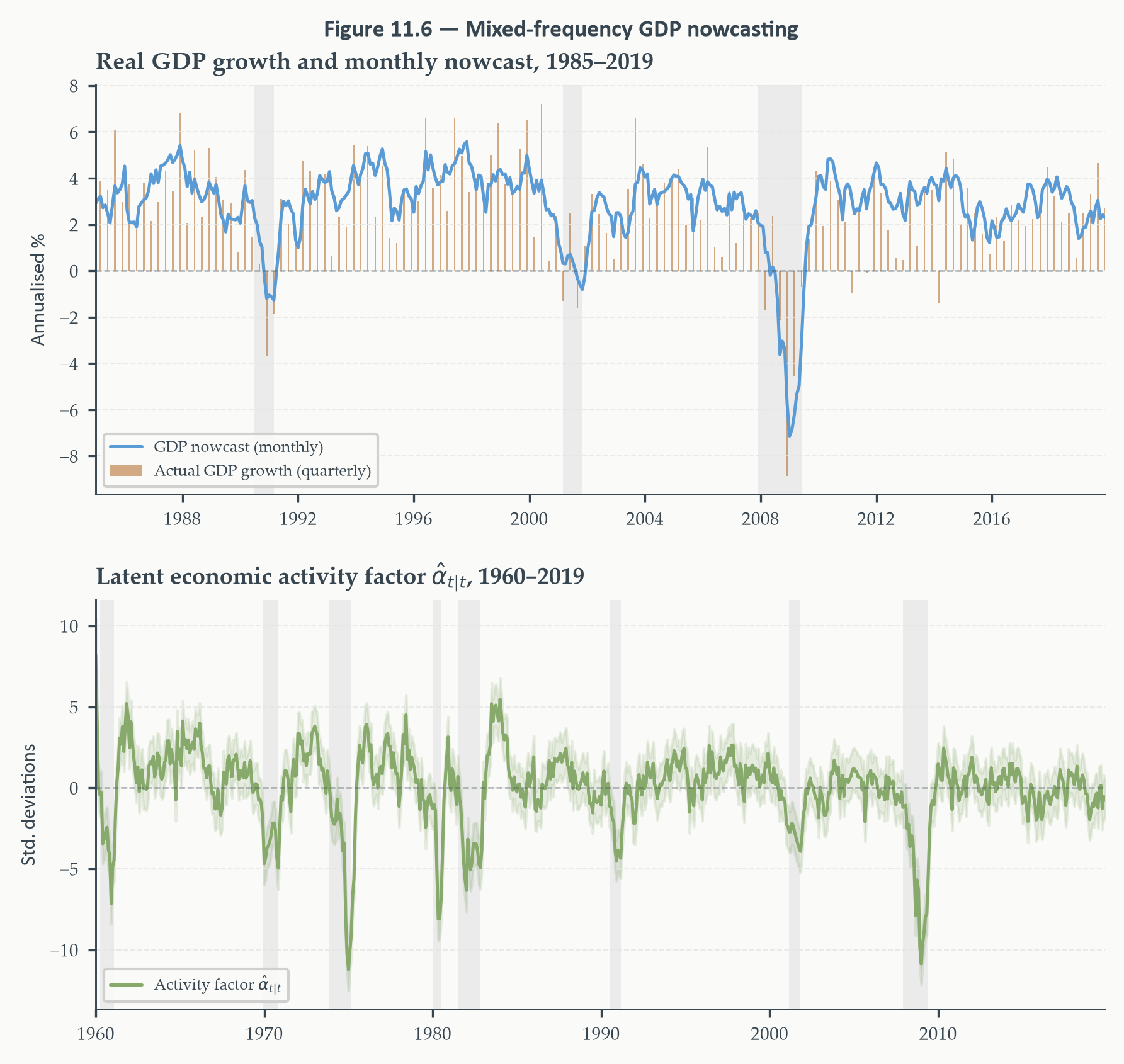
---
title: "State Space Models and the Kalman Filter"
author: ""
abstract: |
Every model in Chapters 1 through 9 assumed that the structure of the data
generating process is fixed — that the parameters governing mean dynamics,
volatility, and long-run relationships are constants that we estimate once
and apply uniformly across the entire sample. This chapter relaxes that
assumption in the most general way available. In the state space framework,
the "state" of the world — trend inflation, a time-varying coefficient, an
unobserved component — is treated as a latent variable that evolves according
to its own dynamics. What we observe is a noisy signal of that state. The
Kalman filter is the algorithm that recovers the best estimate of the hidden
state from the noisy observations, updating in real time as new data arrive.
We begin by showing that the framework is not new: the
GARCH(1,1) recursion of Chapter 9 is already a state equation in disguise,
and the Kalman filter and the GARCH filter share the same
prediction-correction logic. From there we build upward: the local level
model as the pedagogical workhorse, the scalar Kalman recursion derived step
by step, the distinction between filtering and smoothing, and the generalised
matrix form that unifies ARIMA, structural time series, and time-varying
parameter models under a single roof. The running example is monthly core
PCE inflation from 1960 through 2019 — a series whose history of Great
Inflation, Volcker disinflation, and Great Moderation makes the idea of a
slowly drifting, unobserved trend immediately compelling. The chapter closes
by connecting the Kalman filter to nowcasting, showing that the same
recursive updating logic that estimates trend inflation is exactly what
policymakers use to track economic conditions in real time.
jupyter: python3
format:
html:
toc: true
toc-depth: 3
toc-title: "In this chapter"
number-sections: true
code-fold: true
code-summary: "Show code"
code-tools: true
theme: cosmo
css: styles.css
highlight-style: github
fig-align: center
fig-cap-location: bottom
fig-responsive: true
html-math-method: mathjax
embed-resources: false
execute:
echo: true
warning: false
message: false
cache: false
---
```{python}
#| label: setup
#| include: false
import numpy as np
import pandas as pd
import matplotlib.pyplot as plt
import matplotlib as mpl
import matplotlib.ticker as mticker
import pandas_datareader.data as web
import statsmodels.api as sm
from statsmodels.tsa.statespace.structural import UnobservedComponents
from statsmodels.tsa.arima.model import ARIMA
from statsmodels.stats.diagnostic import acorr_ljungbox
from statsmodels.tsa.stattools import acf
from scipy import stats
from datetime import datetime
import warnings
warnings.filterwarnings("ignore")
# ── EO Brand Palette ───────────────────────────────────────────────────────────
EO_CHARCOAL = "#36454F"
EO_COPPER = "#B87333"
EO_SAGE = "#87A96B"
EO_SKYBLUE = "#5B9BD5"
EO_TERRACOTTA = "#D4745E"
EO_LAVENDER = "#8E7AB5"
EO_COLORS = [EO_COPPER, EO_SKYBLUE, EO_SAGE,
EO_TERRACOTTA, EO_LAVENDER, EO_CHARCOAL]
PAGE_BG = "#FAFAF8"
# ── Global rcParams ────────────────────────────────────────────────────────────
mpl.rcParams.update({
"figure.figsize": (6, 3),
"figure.dpi": 150,
"figure.facecolor": PAGE_BG,
"figure.edgecolor": PAGE_BG,
"axes.facecolor": PAGE_BG,
"axes.edgecolor": EO_CHARCOAL,
"axes.linewidth": 0.7,
"axes.grid": True,
"axes.grid.axis": "y",
"axes.spines.top": False,
"axes.spines.right": False,
"axes.titlesize": 9,
"axes.titleweight": "bold",
"axes.titlecolor": EO_CHARCOAL,
"axes.titlelocation": "left",
"axes.labelsize": 8,
"axes.labelcolor": EO_CHARCOAL,
"axes.labelweight": "normal",
"axes.prop_cycle": mpl.cycler(color=EO_COLORS),
"grid.color": "#E5E5E5",
"grid.linewidth": 0.5,
"grid.linestyle": "--",
"grid.alpha": 0.8,
"xtick.color": EO_CHARCOAL,
"ytick.color": EO_CHARCOAL,
"xtick.labelsize": 7,
"ytick.labelsize": 7,
"xtick.direction": "out",
"ytick.direction": "out",
"xtick.major.size": 3,
"ytick.major.size": 3,
"lines.linewidth": 1.2,
"lines.solid_capstyle": "round",
"legend.frameon": True,
"legend.framealpha": 0.9,
"legend.edgecolor": "#CCCCCC",
"legend.facecolor": PAGE_BG,
"legend.fontsize": 6,
"legend.title_fontsize": 6,
"font.family": "serif",
"font.serif": ["Palatino Linotype", "Palatino", "Georgia",
"DejaVu Serif"],
"font.sans-serif": ["Calibri", "Arial", "DejaVu Sans"],
"font.size": 8,
"text.color": EO_CHARCOAL,
"savefig.dpi": 300,
"savefig.bbox": "tight",
"savefig.facecolor": PAGE_BG,
})
def eo_suptitle(fig, title, **kwargs):
defaults = dict(fontsize=9, fontweight="bold",
color=EO_CHARCOAL, fontfamily="Calibri", y=1.01)
defaults.update(kwargs)
fig.suptitle(title, **defaults)
def eo_style_ax(ax):
for obj in [ax.title, ax.xaxis.label, ax.yaxis.label]:
obj.set_fontfamily("Calibri")
# NBER recession dates — extended to cover full 1960–2019 sample
RECESSIONS = [
("1960-04-01", "1961-02-01"),
("1969-12-01", "1970-11-01"),
("1973-11-01", "1975-03-01"),
("1980-01-01", "1980-07-01"),
("1981-07-01", "1982-11-01"),
("1990-07-01", "1991-03-01"),
("2001-03-01", "2001-11-01"),
("2007-12-01", "2009-06-01"),
]
def shade_recessions(ax, start=None, end=None):
for rec_start, rec_end in RECESSIONS:
s, e = pd.Timestamp(rec_start), pd.Timestamp(rec_end)
if start is not None and e < pd.Timestamp(start):
continue
if end is not None and s > pd.Timestamp(end):
continue
ax.axvspan(s, e, color=EO_CHARCOAL, alpha=0.08, lw=0)
```
```{python}
#| label: data-download
#| include: false
#| cache: true
# ── Core PCE inflation via FRED ────────────────────────────────────────────────
# PCEPILFE: Personal Consumption Expenditures Excluding Food and Energy
# (Chain-Type Price Index), monthly, seasonally adjusted, index 2012=100.
# We compute annualised month-on-month log changes and restrict to
# 1960-01 through 2019-12. The pre-COVID restriction follows the convention
# established in Chapters 4–9: the pandemic represents a structural break of
# unusual severity that would distort any model estimated on normal business
# cycle dynamics. Annualised changes (multiplied by 12) put the series in
# familiar percent-per-year units; the alternative of year-on-year changes
# introduces a 12-month moving average effect that would bias the local level
# model's signal extraction.
from pathlib import Path
DATA_PATH = Path("../../data/raw")
pce_raw = pd.read_csv(DATA_PATH / "PCEPILFE.csv", index_col="date", parse_dates=True).loc["1959-12-01":"2019-12-01"]
pce_raw.columns = ["PCE_Level"]
# Annualised month-on-month percent change: 12 * 100 * Δlog(P)
pce_raw["Inflation"] = np.log(pce_raw["PCE_Level"]).diff() * 100 * 12
# Drop the first observation (NaN after differencing); restrict sample
pce = pce_raw.loc["1960-01-01":"2019-12-01", ["Inflation"]].dropna().copy()
pce.index = pd.to_datetime(pce.index)
SAMPLE_START = pce.index[0].strftime("%Y-%m-%d")
SAMPLE_END = pce.index[-1].strftime("%Y-%m-%d")
N_OBS = len(pce)
# Convenience arrays used throughout
inflation = pce["Inflation"].values
dates = pce.index
```
::: {.callout-note}
## Learning Objectives
By the end of this chapter, you will be able to:
- Explain why the GARCH(1,1) variance recursion is already a state equation in
disguise, and use this connection to motivate the state space framework as a
generalisation of tools already in your toolkit
- Write down the observation equation and state equation of the local level
model, and give an economic interpretation of each noise term
- Derive the Kalman filter recursion step by step in scalar form: the prediction
step, the Kalman gain, and the update step
- Explain the role of the signal-to-noise ratio in governing how quickly the
filter responds to new data, and interpret its estimated value on real data
- Distinguish between the filtered estimate, the smoothed estimate, and the
forecast of a latent state variable, and explain when each is the appropriate
object of interest
- Fit a local level model in Python using `statsmodels.tsa.statespace`,
extract filtered and smoothed trend estimates, and produce a fan chart forecast
- Map ARIMA models, exponential smoothing, and time-varying parameter
regressions onto the general state space form, recognising them as special
cases of a single framework
- Describe what nowcasting is, explain why the Kalman filter is the natural
tool for it, and illustrate recursive state updating on a real series
:::
Chapter 9 closed with a question: what if the parameters of a volatility model
are not constant across time? That question opens the door to the state space
framework, the most general modelling architecture introduced in this book.
Section 11.1 begins by honouring the bridge from Chapter 9: the GARCH(1,1)
variance recursion, reread carefully, is already a state equation — the
conditional variance is an unobserved state, and the squared return is a noisy
observation of it. That reinterpretation motivates the general vocabulary of
observation equations, state equations, and the signal-noise decomposition.
Section 11.2 introduces the local level model: the simplest non-trivial state
space model, and the one that does most of the pedagogical work in this chapter.
Section 11.3 derives the Kalman filter from scratch in scalar form, walking
through the prediction and update steps with enough algebra to make the
recursion completely transparent. Section 11.4 addresses practical matters —
initialisation, the signal-to-noise ratio, and how the filter is estimated from
data. Section 11.5 sharpens the distinction between filtering, smoothing, and
forecasting. Section 11.6 presents the general matrix form of the state space
model and shows that ARIMA, exponential smoothing, and time-varying parameter
regressions are all special cases. Section 11.7 applies the full apparatus to
core PCE inflation, tracing the Great Inflation and the [Great Moderation](https://en.wikipedia.org/wiki/Great_Moderation) through
a smoothed trend estimate. Section 11.8 connects the Kalman filter to
nowcasting. Throughout, the running example is monthly core PCE inflation from
1960 through 2019.
## From GARCH to State Space: The Unifying Idea {#sec-garch-ss}
### A Recursion You Already Know
Chapter 9 left us with a model — the GARCH(1,1) — that is both powerful and
somewhat mysterious. We can write it down, estimate it, and interpret its
parameters, but the mechanism by which it tracks volatility over time still
feels opaque. Why does the GARCH filter work? What principle is it
implementing? And why does it do a good job of recovering an object —
conditional variance — that we never directly observe?
The answer lies in a reinterpretation that reveals the GARCH(1,1) to be a
member of a much larger family. Write the GARCH variance recursion again:
$$\sigma_t^2 = \omega + \alpha \varepsilon_{t-1}^2 + \beta \sigma_{t-1}^2 \tag{10.1}$$
Now ask: what role does each object play? The conditional variance $\sigma_t^2$
is not observed — it is inferred from data, not measured directly. The squared
return $\varepsilon_{t-1}^2$ is observed, but it is a noisy proxy for
$\sigma_{t-1}^2$: even if we knew the true variance, the realised squared
return in any given period would deviate from it because of the random shock
$z_{t-1}^2$. And the recursion (10.1) is predicting today's hidden
variance using yesterday's hidden variance plus a correction based on
yesterday's noisy signal.
This is the prediction-correction structure that the Kalman filter implements.
To make it precise, rewrite the squared return as:
$$\varepsilon_t^2 = \sigma_t^2 \cdot z_t^2 \tag{10.2}$$
where $z_t \sim \text{i.i.d.}(0,1)$. Taking expectations,
$\mathbb{E}[\varepsilon_t^2 \mid \mathcal{F}_{t-1}] = \sigma_t^2$. So
$\varepsilon_t^2$ is an unbiased but noisy observation of the latent variance
$\sigma_t^2$, with a multiplicative noise term $z_t^2$ that has mean one and
variance two (for standard normal $z_t$). In this light, equation (10.1) is
not just a variance model — it is an algorithm for extracting a signal from a
noisy measurement.
::: {.callout-note icon=false}
## Definition 11.1 — State Variable and Observation
A **state variable** is an unobserved quantity that summarises all
past-relevant information about the system at time $t$. In the GARCH(1,1),
the state variable is the conditional variance $\sigma_t^2$. An
**observation** is a measured quantity that depends on the current state plus
noise. In the GARCH(1,1), the observation is the squared return
$\varepsilon_t^2 = \sigma_t^2 z_t^2$.
:::
### The Two-Equation Structure
The state space framework formalises this two-layer structure with two
equations. The **observation equation** describes how what we measure relates
to the underlying state:
$$y_t = f(\alpha_t) + \text{observation noise} \tag{10.3}$$
The **state equation** describes how the unobserved state evolves over time:
$$\alpha_t = g(\alpha_{t-1}) + \text{state noise} \tag{10.4}$$
In the GARCH(1,1), the observation equation is $\varepsilon_t^2 = \sigma_t^2
z_t^2$ — the state enters the observation multiplicatively, with noise $z_t^2
- 1$. The state equation is the GARCH recursion itself (10.1) — the state
evolves as a weighted combination of the previous state and the previous
observation, with no additive noise term. GARCH has a deterministic state
equation, which is a restriction we will relax in the next section.
This is the structure that defines every state space model, and the Kalman
filter is the algorithm that solves the inference problem it poses: given the
sequence of observations $y_1, \ldots, y_t$, what is our best estimate of the
current state $\alpha_t$?
### What GARCH Cannot Do — and Why That Matters
The GARCH(1,1) is a special case of the state space framework with two
important restrictions. First, the state equation is deterministic:
$\sigma_t^2$ is a fixed function of past data, with no random shock of its
own. Second, the parameters $\omega$, $\alpha$, and $\beta$ are constants —
the volatility-clustering mechanism operates with the same intensity in every
period.
Chapter 9's Looking Ahead section asked what happens when these restrictions
are lifted. What if the unconditional variance $\omega/(1-\alpha-\beta)$ shifts
over time, as it plausibly did between the volatile 1970s and the calm Great
Moderation? What if the parameters $\alpha$ and $\beta$ themselves drift?
The state space framework answers this question directly. When the state
equation includes its own noise term — when the state can move randomly rather
than following a fixed recursion — the model allows the underlying structure to
evolve. The Kalman filter then estimates both the current state *and* its
uncertainty, updating both as new observations arrive. GARCH is a state space
model without state noise. The local level model, which we develop in the next
section, is the simplest example of what happens when we add it.
::: {.callout-note icon=false}
## The Prediction-Correction Principle
Both the GARCH filter and the Kalman filter implement the same two-step logic
at every period:
1. **Predict**: use the state equation to project the hidden state one period
forward, together with its uncertainty.
2. **Correct**: observe the new data point; compute how far the observation
deviates from the prediction; update the state estimate by weighting the
prediction against the new signal.
The weight assigned to the new signal relative to the prior prediction depends
on how noisy the observation is relative to how uncertain the prediction is.
When observations are very noisy, the filter trusts the prediction and updates
little. When observations are precise relative to the prior uncertainty, the
filter updates aggressively. The GARCH gain parameter $\alpha$ is a fixed
version of this weight. The Kalman gain, which we derive in Section 11.3, is
the time-varying optimal version.
:::
### A First Glimpse: Tracking Inflation in the 1970s
Before formalising any of this, a concrete example fixes the ideas. It is
early 1975. The Federal Reserve is trying to assess the state of underlying
inflation after the first oil shock. Monthly readings of core PCE have been
coming in all over the place — annualised month-on-month changes of 4, 9, 7,
11, 6 percent in consecutive months. None of these individual readings is
"trend inflation." Each is trend inflation plus noise: transitory supply
disruptions, seasonal residuals, data revisions, measurement error. What the
Fed wants to know is the hidden state — the persistent underlying inflation
pressure that monetary policy actually needs to respond to.
Suppose, based on everything observed up to December 1974, our best estimate
of trend inflation is $\hat{\mu}_{t-1} = 7.5$ percent, and we are moderately
uncertain about it, with a standard deviation of 1.2 percent around that
estimate. Now January 1975 arrives and the reported core PCE inflation reading
is $y_t = 11.4$ percent — a large number, well above our prior estimate.
Two extreme responses are both wrong. We could ignore the new reading entirely
and keep our estimate at 7.5 — but that discards genuinely informative data.
Or we could update all the way to 11.4 — but that treats one noisy monthly
number as a perfect signal of underlying inflation, which it is not. The right
answer lies somewhere in between, and the weight depends on a single question:
how noisy is the monthly reading relative to how uncertain we already are about
the state?
If monthly inflation is very noisy relative to our prior uncertainty — if the
observation standard deviation is, say, 3.0 percent — then the new reading
moves our estimate only modestly, say to 8.7 percent. The prior dominates.
If the monthly reading is relatively precise — observation standard deviation
of 0.8 percent — then the new reading carries more weight and our estimate
moves further, say to 10.6 percent. The Kalman gain is the formula that
computes this weight optimally. We derive it in Section 11.3; for now the
intuition is what matters.
Notice also what happens to uncertainty after the update. Before observing
$y_t$, we had a 1.2 percent standard deviation on our state estimate. After
observing $y_t$ and incorporating it — regardless of whether it pushes our
estimate up or down — our uncertainty about the state should be *smaller*,
because we now know more. The Kalman filter tracks this uncertainty reduction
period by period alongside the state estimate itself. This is the feature that
distinguishes it from the GARCH filter, which produces a point estimate of
variance but no explicit measure of estimation uncertainty.
This two-number summary — a state estimate and an uncertainty measure — is
what flows forward into the next period's prediction step. January's posterior
becomes February's prior. The filter is a machine for converting a sequence
of noisy observations into a sequence of progressively refined state estimates,
each carrying its own measure of how confident we should be. Section 11.2
writes this down precisely for the simplest possible case.
## The Local Level Model {#sec-llm}
The inflation example in Section 11.1 had all the ingredients of a state space
model: an unobserved trend, noisy monthly observations, and a question about
how the trend evolves. The **local level model** is the minimal formal
structure that captures exactly this. It has two equations and two parameters,
and almost everything important about the Kalman filter can be seen in it
before we ever write down a matrix.
The economic premise is simple. Suppose the "true" level of some series —
trend inflation, say — drifts over time in a way that is not fully predictable.
Each period, it moves by a small random amount. What we observe is this drifting
level plus measurement noise. Our task is to recover the hidden level from the
noisy observations.
### The Model
Let $y_t$ be the observed series (monthly core PCE inflation, in annualised
percent) and $\mu_t$ be the unobserved trend. The local level model is:
$$y_t = \mu_t + \varepsilon_t, \qquad \varepsilon_t \sim \text{i.i.d.}(0,\, \sigma_\varepsilon^2) \tag{10.5}$$
$$\mu_t = \mu_{t-1} + \eta_t, \qquad \eta_t \sim \text{i.i.d.}(0,\, \sigma_\eta^2) \tag{10.6}$$
with $\varepsilon_t$ and $\eta_t$ independent of each other and of all past
values. Equation (10.5) is the **observation equation**: the observed inflation
reading equals the latent trend plus measurement noise $\varepsilon_t$.
Equation (10.6) is the **state equation**: the trend itself evolves as a
random walk, drifting by a shock $\eta_t$ each period.
::: {.callout-note icon=false}
## Definition 11.2 — The Local Level Model
The **local level model** is the state space model defined by equations
(10.5) and (10.6). It is characterised by two variance parameters:
- $\sigma_\varepsilon^2$: the **observation variance** — how noisy the
measured series is around the true underlying level.
- $\sigma_\eta^2$: the **state variance** — how much the underlying level
itself moves from period to period.
Everything about the model's behaviour is governed by the ratio of these two
variances, which we examine in detail in Section 11.4.
:::
The economic interpretation is immediate. Inflation in any given month is not
just trend inflation — it is trend inflation plus the noise of a single monthly
price survey, seasonal residuals not fully removed by the seasonal adjustment
procedure, transitory supply-side shocks, and measurement error. The
observation equation separates these two contributions. The state equation says
that trend inflation itself is not fixed: it drifted upward through the 1970s
as the Fed's credibility eroded, fell sharply in the early 1980s as Volcker
tightened policy, and settled into a stable 2 percent range during the Great
Moderation. The $\eta_t$ shocks are the forces — policy shifts, supply shocks
with persistent effects, changes in inflation expectations — that move trend
inflation from one period to the next.
### Connecting to Models You Already Know
The local level model is not new. It is a formal statement of something we
already encountered twice in earlier chapters, in different guises.
First, look at the observation equation (10.5) alone. If the trend $\mu_t$
were constant — if $\sigma_\eta^2 = 0$ — the model reduces to a fixed mean
plus i.i.d. noise: $y_t = \mu + \varepsilon_t$. That is just the white noise
model of Chapter 1. The state equation (10.6) is the generalisation that
allows the mean to drift.
Second, consider what happens at the other extreme: if $\sigma_\varepsilon^2
= 0$, so that there is no observation noise, then $y_t = \mu_t$ exactly, and
the state equation says $y_t = y_{t-1} + \eta_t$ — a pure random walk. We
studied this in Chapter 4 as the canonical I(1) process. The local level model
nests both the stationary mean model and the pure random walk as boundary
cases.
Third — and most directly useful for project work — Chapter 2 introduced
exponential smoothing as a heuristic forecasting device. The update rule of
Holt's simple exponential smoothing is:
$$\hat{\mu}_t = (1-\lambda)\hat{\mu}_{t-1} + \lambda y_t$$
for some smoothing parameter $\lambda \in (0,1)$. It turns out that this rule
is exactly the Kalman filter applied to the local level model, once the filter
has converged to its steady state. The smoothing parameter $\lambda$ is not
arbitrary — it is the steady-state Kalman gain, determined by the
signal-to-noise ratio $q = \sigma_\eta^2 / \sigma_\varepsilon^2$. The state
space framework gives the heuristic of Chapter 2 a rigorous derivation and
a statistical interpretation. We return to this connection in Section 11.4.
::: {.callout-warning icon=false}
## The Random Walk Trend Is Not the Same as Nonstationarity
The state equation $\mu_t = \mu_{t-1} + \eta_t$ looks like a unit root
process, and in a narrow sense it is. But the *observed* series $y_t = \mu_t
+ \varepsilon_t$ is not simply I(1): it is the sum of an I(1) component and
an I(0) component, which makes it an integrated moving average — specifically,
an ARIMA(0,1,1) process. This is not a contradiction; it reflects the
fact that the local level model imposes structure on *how* the unit root
enters the data. The ADF and KPSS tests of Chapter 4 applied to $y_t$ will
typically fail to reject a unit root, which is consistent with the model — but
the local level decomposition tells us something ADF cannot: how much of the
apparent nonstationarity is permanent trend drift versus transitory observation
noise.
:::
### What We Need to Estimate
The local level model has two unknown parameters: $\sigma_\varepsilon^2$ and
$\sigma_\eta^2$. In principle, estimating them is a standard statistical
problem — we have a sample of $T$ observations $y_1, \ldots, y_T$ and we want
to choose $(\sigma_\varepsilon^2, \sigma_\eta^2)$ to best fit the data.
The complication is that the likelihood of the data under the local level model
is not a simple closed-form expression. The latent states $\mu_1, \ldots,
\mu_T$ are unobserved, so they must be integrated out. The Kalman filter
solves this problem as a by-product of its state estimation: running the filter
forward through the data produces the prediction errors (called **innovations**)
that enter the likelihood, and those innovations can be evaluated at any
candidate parameter values. Maximising the resulting **prediction error
decomposition** of the likelihood over $(\sigma_\varepsilon^2, \sigma_\eta^2)$
gives maximum likelihood estimates. We return to estimation in Section 11.4
after deriving the filter itself.
## The Kalman Filter {#sec-kalman}
### The Inference Problem
We now have a model — the local level model — and a question: given
observations $y_1, \ldots, y_t$, what is the best estimate of the current
state $\mu_t$? "Best" here means minimum mean squared error: we want the
estimate $\hat{\mu}_{t|t}$ that minimises $\mathbb{E}[(\mu_t -
\hat{\mu}_{t|t})^2]$.
The subscript notation is important and worth fixing precisely. We write:
- $\hat{\mu}_{t|t-1}$: the **predicted state** — our best estimate of $\mu_t$
using only information up to and including $t-1$, before seeing $y_t$.
- $\hat{\mu}_{t|t}$: the **filtered state** — our best estimate of $\mu_t$
after incorporating $y_t$.
- $P_{t|t-1}$: the **predicted variance** — the mean squared error of
$\hat{\mu}_{t|t-1}$.
- $P_{t|t}$: the **filtered variance** — the mean squared error of
$\hat{\mu}_{t|t}$.
The [Kalman filter](https://en.wikipedia.org/wiki/Kalman_filter) is the recursive algorithm that computes all four of these
objects period by period, starting from an initial condition and updating as
new observations arrive.
### The Recursion: Two Steps
#### Step 1 — Prediction
At the start of period $t$, we know $\hat{\mu}_{t-1|t-1}$ and $P_{t-1|t-1}$
from the previous period. The state equation says $\mu_t = \mu_{t-1} + \eta_t$
with $\eta_t \sim (0, \sigma_\eta^2)$. Taking expectations:
$$\hat{\mu}_{t|t-1} = \hat{\mu}_{t-1|t-1} \tag{10.7}$$
The best prediction of where the trend is today is where it was yesterday —
because the shock $\eta_t$ has mean zero and is not yet observable. The
prediction variance picks up the additional uncertainty from the state shock:
$$P_{t|t-1} = P_{t-1|t-1} + \sigma_\eta^2 \tag{10.8}$$
Notice that only $\sigma_\eta^2$ — the state noise variance — appears here.
The observation noise $\sigma_\varepsilon^2$ plays no role in the prediction
step because observations have not yet arrived: we are projecting the state
forward using only the state equation, which carries $\eta_t$ but not
$\varepsilon_t$. The observation noise enters one step later, in the
innovation variance (10.10), once $y_t$ is in hand. This separation between
the two noise sources — state noise inflates the predicted variance, observation
noise inflates the innovation variance — is a key structural feature of the
recursion.
Our uncertainty about the state grows by $\sigma_\eta^2$ each period that we
go without a new observation. This is the cost of a drifting state: unlike a
fixed parameter, the trend can move between observations, so the further we
are from the last data point, the more uncertain we are about where the trend
currently sits.
#### Step 2 — Update
Now $y_t$ arrives. The **innovation** — the surprise in $y_t$ relative to
what we predicted — is:
$$v_t = y_t - \hat{\mu}_{t|t-1} \tag{10.9}$$
The innovation variance — how much uncertainty there is in this surprise — is:
$$F_t = P_{t|t-1} + \sigma_\varepsilon^2 \tag{10.10}$$
It combines prediction uncertainty $P_{t|t-1}$ (we are not sure where the
trend is) with observation noise $\sigma_\varepsilon^2$ (even if we knew the
trend perfectly, the observation would still deviate from it). The
**Kalman gain** is:
$$K_t = \frac{P_{t|t-1}}{F_t} = \frac{P_{t|t-1}}{P_{t|t-1} + \sigma_\varepsilon^2} \tag{10.11}$$
The gain $K_t \in (0,1)$ measures how much weight the filter places on the
new observation relative to the prior prediction. We update:
$$\hat{\mu}_{t|t} = \hat{\mu}_{t|t-1} + K_t \, v_t \tag{10.12}$$
$$P_{t|t} = (1 - K_t)\, P_{t|t-1} \tag{10.13}$$
Equation (10.12) is the prediction-correction principle in algebra: the
filtered estimate is the predicted estimate plus a fraction $K_t$ of the
surprise. Equation (10.13) says that incorporating an observation always
reduces our uncertainty — $P_{t|t} < P_{t|t-1}$ for any $K_t > 0$ — because
any signal, however noisy, is informative.
::: {.callout-note icon=false}
## The Kalman Gain in Plain Language
The Kalman gain $K_t = P_{t|t-1} / (P_{t|t-1} + \sigma_\varepsilon^2)$ is the
ratio of prediction uncertainty to total uncertainty. Two extremes are
instructive:
- If $\sigma_\varepsilon^2 \to \infty$ (observations are pure noise), then
$K_t \to 0$: the filter ignores the new observation entirely and keeps the
prior.
- If $\sigma_\varepsilon^2 \to 0$ (observations are perfect measurements),
then $K_t \to 1$: the filter sets $\hat{\mu}_{t|t} = y_t$, trusting the
observation completely.
In practice $K_t$ lies between these extremes, and its value — determined by
the relative magnitudes of state and observation noise — encodes a precise
answer to the question: how much should we revise our beliefs in response to
a single new data point?
:::
### A Numerical Example: Filtering Inflation in January 1975
We return to the January 1975 scenario from Section 11.1, now with the algebra
in hand. Suppose the model parameters (estimated from pre-1975 data) are
$\sigma_\varepsilon^2 = 4.0$ (percent$^2$, annualised) and $\sigma_\eta^2 =
0.5$. The filtered state from December 1974 is $\hat{\mu}_{t-1|t-1} = 7.5$
percent with filtered variance $P_{t-1|t-1} = 1.44$ (standard deviation 1.2
percent). The January 1975 observation is $y_t = 11.4$ percent.
**Prediction step.** We project the state forward:
$$\hat{\mu}_{t|t-1} = 7.5 \qquad P_{t|t-1} = 1.44 + 0.5 = 1.94$$
Our prior uncertainty grows slightly because the trend may have drifted during
January.
**Innovation.** The surprise in the new observation is:
$$v_t = 11.4 - 7.5 = 3.9 \text{ percentage points}$$
That is a large surprise — nearly 4 percentage points above our predicted
trend. But before revising strongly upward, we need to know how much weight
to put on it.
**Kalman gain.** The innovation variance is:
$$F_t = 1.94 + 4.0 = 5.94$$
The Kalman gain is:
$$K_t = \frac{1.94}{5.94} \approx 0.327$$
The filter assigns roughly one-third of the weight to the new observation and
two-thirds to the prior. The observation noise $\sigma_\varepsilon^2 = 4.0$
is large relative to the prediction variance $P_{t|t-1} = 1.94$, so the
filter is appropriately sceptical of a single monthly reading.
**Update step.** The filtered state and variance are:
$$\hat{\mu}_{t|t} = 7.5 + 0.327 \times 3.9 = 7.5 + 1.28 = 8.78 \text{ percent}$$
$$P_{t|t} = (1 - 0.327) \times 1.94 = 0.673 \times 1.94 = 1.31$$
We revise our estimate of trend inflation upward from 7.5 to 8.78 percent —
a meaningful move, but well short of the noisy 11.4 reading. Our uncertainty
falls from a standard deviation of $\sqrt{1.94} \approx 1.39$ to
$\sqrt{1.31} \approx 1.14$ percent: January's observation has reduced our
uncertainty about the trend, even though it was itself noisy.
In February, $\hat{\mu}_{t|t} = 8.78$ and $P_{t|t} = 1.31$ become the new
prior, and the recursion repeats. Period by period, the filter assembles a
complete history of trend inflation — not a single static estimate, but a
time-varying sequence of best guesses, each with its own uncertainty.
### The Recursion in Motion
The single-step example above is enough to understand the algebra. But to
see why the recursion matters — why running it for twelve consecutive months
produces something qualitatively different from any single update — it helps
to watch the filter work through a full year.
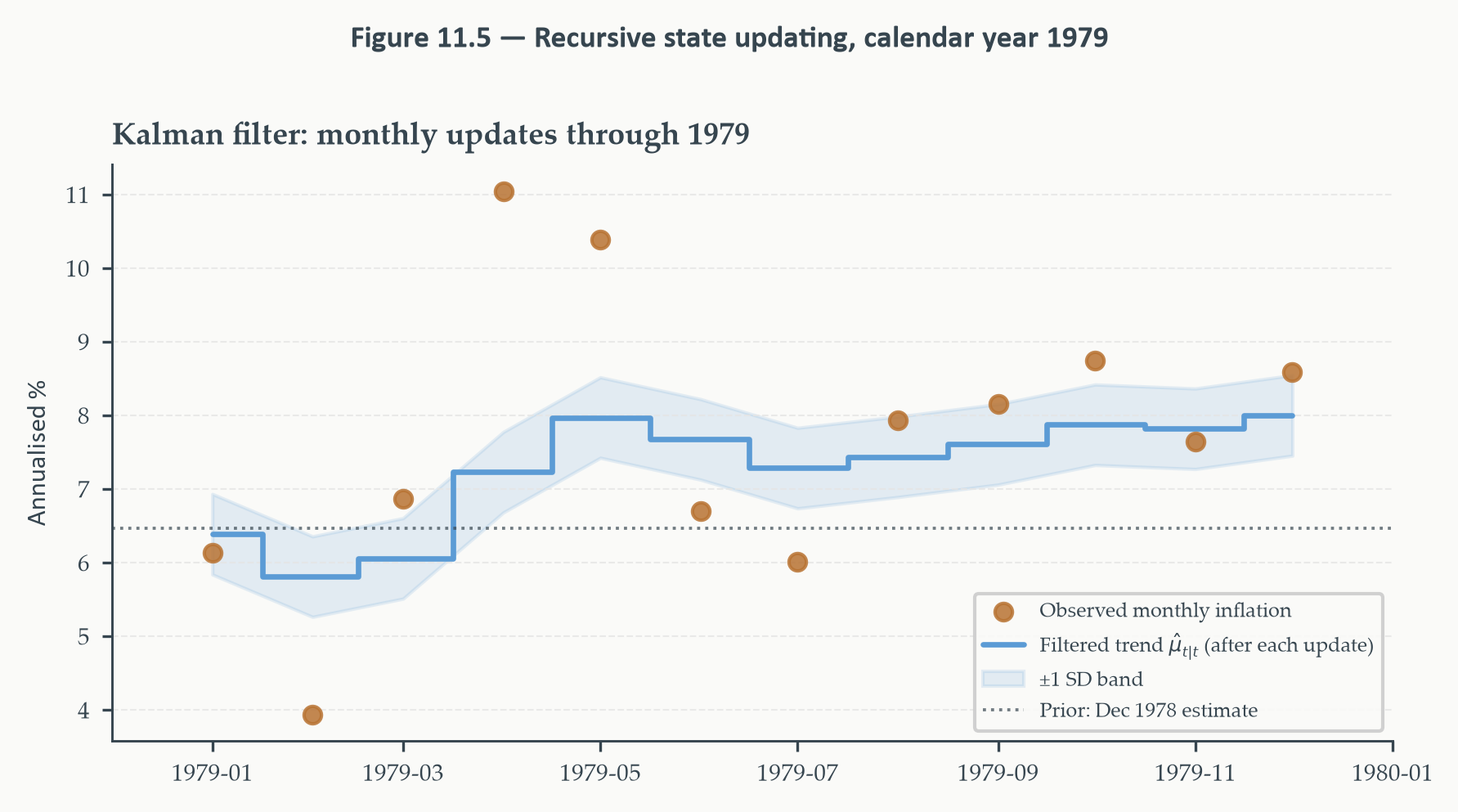
Figure 11.5 traces the filter through all twelve months of 1979, a year in
which observed inflation was running well above any plausible prior estimate
of the trend. Each month, a new observation arrives, a new Kalman gain is
computed, and the trend estimate is revised. The figure shows the cumulative
effect: twelve updates, each modest on its own, that together shift the
filter's reading of trend inflation substantially upward. The prediction-
correction loop is the same each period — predict, observe, update — but the
accumulated evidence gradually overrides the prior.
```{python}
#| label: fig-recursive-updating
#| fig-cap: "**The Kalman filter in motion: twelve consecutive updates through
#| 1979.** Copper dots: observed monthly core PCE inflation (annualised).
#| Sky blue step line: filtered trend estimate $\\hat{\\mu}_{t|t}$ after
#| each successive monthly update. Dotted horizontal line: the December 1978
#| prior. Each step reflects one prediction-correction cycle; the cumulative
#| effect of twelve updates shifts the trend estimate well above the prior
#| as the filter accumulates evidence that the rise in inflation is
#| persistent, not transitory."
# ── Self-contained fit to obtain parameters and Dec 1978 posterior ────────────
# Section 11.7 fits and interprets the full model; this cell fits it silently
# here so Figure 11.5 does not depend on Section 11.7's execution order.
# Underscore-prefixed names avoid collision with Section 11.7 variables.
_llm_early  = UnobservedComponents(pce["Inflation"], level="local level")
_llm_fit    = _llm_early.fit(disp=False)
_s2_eps     = _llm_fit.params["sigma2.irregular"]
_s2_eta     = _llm_fit.params["sigma2.level"]
_fstate     = _llm_fit.filtered_state[0]
_fvar       = _llm_fit.filtered_state_cov[0, 0]

# ── Recursive updating illustration for calendar year 1979 ────────────────────
idx_start = pce.index.get_loc("1979-01-01")
idx_end   = pce.index.get_loc("1979-12-01")
idx_prior = pce.index.get_loc("1978-12-01")

mu_prior = _fstate[idx_prior]
P_prior  = _fvar[idx_prior]

months_1979 = dates[idx_start : idx_end + 1]
obs_1979    = inflation[idx_start : idx_end + 1]

mu_seq, P_seq = [], []
mu_t, P_t = mu_prior, P_prior

for y_t in obs_1979:
    mu_pred = mu_t
    P_pred  = P_t + _s2_eta
    v_t     = y_t - mu_pred
    F_t     = P_pred + _s2_eps
    K_t     = P_pred / F_t
    mu_t    = mu_pred + K_t * v_t
    P_t     = (1 - K_t) * P_pred
    mu_seq.append(mu_t)
    P_seq.append(P_t)

mu_seq = np.array(mu_seq)
se_seq = np.sqrt(np.array(P_seq))

fig, ax = plt.subplots(figsize=(6, 3.2))

ax.scatter(months_1979, obs_1979,
           color=EO_COPPER, s=26, zorder=5, alpha=0.85,
           label="Observed monthly inflation")
ax.step(months_1979, mu_seq,
        color=EO_SKYBLUE, lw=1.6, where="mid",
        label=r"Filtered trend $\hat{\mu}_{t|t}$ (after each update)")
ax.fill_between(months_1979,
                mu_seq - se_seq,
                mu_seq + se_seq,
                color=EO_SKYBLUE, alpha=0.15,
                label="±1 SD band")
ax.axhline(mu_prior, color=EO_CHARCOAL, lw=0.9, ls=":",
           alpha=0.7, label="Prior: Dec 1978 estimate")

ax.set_xlim(months_1979[0] - pd.DateOffset(months=1),
            months_1979[-1] + pd.DateOffset(months=1))
ax.set_ylabel("Annualised %")
ax.set_title("Kalman filter: monthly updates through 1979")
ax.legend(loc="lower right", fontsize=6)
eo_style_ax(ax)
eo_suptitle(fig, "Figure 11.5 — Recursive state updating, calendar year 1979")

fig.tight_layout()
plt.show()
```
*Figure 11.5 shows the filter working through all twelve months of 1979.
The December 1978 prior sits at approximately 6.5 percent (dotted line).
The January reading comes in close to the prior and produces only a modest
upward revision, but the February observation falls sharply to around 4 percent
-- well below the predicted trend -- pulling the filtered estimate briefly
downward. From March onward the observations run consistently above the
predicted trend, and each successive update pushes the estimate higher.
By December the filtered trend has risen to around 8 percent -- a cumulative
upward revision of roughly 1.5 percentage points from the prior. The ±1 SD
band narrows modestly across the year as twelve monthly observations
progressively reduce uncertainty about where the trend sits. The figure
makes the prediction-correction logic tangible: no single observation is
decisive, but the weight of consistent evidence gradually overrides the prior.*
### What Makes This Optimal?
The [Kalman filter](https://en.wikipedia.org/wiki/Kalman_filter) is not just a plausible updating rule — it is the
minimum-mean-squared-error estimator of the state, given the model. Under the
assumption that $\varepsilon_t$ and $\eta_t$ are Gaussian, it is also the
exact conditional expectation: $\hat{\mu}_{t|t} = \mathbb{E}[\mu_t \mid
y_1, \ldots, y_t]$. With non-Gaussian innovations, it remains the best
*linear* estimator, a property known as the linear minimum variance result.
The derivation of optimality is elegant but algebraically involved. The key
insight is that the joint distribution of $(y_1, \ldots, y_t, \mu_t)$ is
multivariate normal under Gaussian assumptions, and the conditional
expectation of $\mu_t$ given the observations is then a linear function of
those observations — exactly the function the Kalman recursion implements. We
do not work through the full proof here; the important thing is that the gain
formula (10.11) is not an ad hoc choice but a derived result.
::: {.callout-warning icon=false}
## The Filter Requires Correct Parameter Values
The [Kalman filter](https://en.wikipedia.org/wiki/Kalman_filter) recursion (10.7)–(10.13) takes $\sigma_\varepsilon^2$ and
$\sigma_\eta^2$ as given. In the numerical example above, we assumed specific
values for illustration. In practice these parameters are unknown and must be
estimated from the data. Section 11.4 explains how maximum likelihood
estimation via the prediction error decomposition accomplishes this. A
misspecified signal-to-noise ratio leads to a suboptimal gain — the filter
either over-reacts to noisy observations or under-reacts to genuine state
changes. Getting the parameters right is not a technical formality; it
determines the quality of the state estimates.
:::
## Initialisation, the Signal-to-Noise Ratio, and Estimation {#sec-snr}
### Where Does the Filter Start?
The Kalman recursion (10.7)–(10.13) is a forward iteration: each period's
filtered estimate feeds into the next period's prediction. But to start the
machine, we need an initial state estimate $\hat{\mu}_{0|0}$ and an initial
variance $P_{0|0}$ before any data have been observed.
Two approaches are standard. The first is a **diffuse prior**: set
$P_{0|0}$ to a very large number — effectively infinity — signalling that we
have no prior information about the initial level of the trend. In practice
this means setting $P_{0|0} = \kappa$ for a large constant $\kappa$, say
$10^6$. The Kalman gain in the first period is then approximately 1 — the
filter trusts the first observation almost entirely — and the filtered
variance falls rapidly over the first handful of periods as the filter
accumulates information. After roughly $5$–$10$ periods the initial condition
has almost no influence on the filtered states; the filter has "forgotten"
where it started.
The second approach is a **stationary initialisation**: if the model has a
stationary unconditional distribution for the state, set $\hat{\mu}_{0|0}$
equal to the unconditional mean and $P_{0|0}$ equal to the unconditional
variance. This is not available for the local level model because the state
equation $\mu_t = \mu_{t-1} + \eta_t$ is a random walk — it has no
unconditional mean to initialise from. The diffuse prior is therefore the
standard choice for the local level model, and it is what `statsmodels` uses
by default.
::: {.callout-warning icon=false}
## Burn the First Few Observations
When using the diffuse prior, the filtered states and variances in the first
few periods are heavily influenced by the initialisation and should be treated
with caution. For the core PCE application with $T = 720$ monthly observations,
this is a minor concern — the filter converges within the first dozen periods,
which represents less than two years of data at the start of the sample. For
shorter series, the initialisation matters more, and it is worth examining
how sensitive the early filtered states are to the choice of $\kappa$.
:::
### The Signal-to-Noise Ratio
Everything about the local level model's behaviour is governed by a single
dimensionless number: the **signal-to-noise ratio**
$$q = \frac{\sigma_\eta^2}{\sigma_\varepsilon^2} \tag{10.14}$$
This ratio compares how much the hidden state moves each period (state
variance) to how noisy each observation is (observation variance). It is the
single most important quantity in any state space model, and developing
intuition for it is worth some effort.
When $q$ is small — say $q = 0.01$ — the trend barely moves from period to
period, while each monthly observation is comparatively noisy. The filter
should barely react to new data: the prior is much more reliable than any
individual reading. When $q$ is large — say $q = 1.0$ — the trend is volatile
and monthly observations are relatively precise. The filter should update
aggressively, following the data closely.
This intuition is made precise by the **steady-state Kalman gain**. For the
local level model, the filter variance $P_{t|t-1}$ converges to a fixed value
$\bar{P}$ as $t \to \infty$. To find it, we impose the steady-state condition
$P_{t|t-1} = P_{t-1|t-1} \equiv \bar{P}$ in the two-step recursion — that is,
we require the predicted variance to be the same from one period to the next.
Substituting into (10.8) and (10.13) and solving the resulting quadratic in
$\bar{P}$ yields a unique positive root. Substituting that root back into
(10.11) gives the steady-state Kalman gain:
$$\bar{K} = \frac{-q + \sqrt{q^2 + 4q}}{2} \tag{10.15}$$
The formula can be understood geometrically without algebra. In steady state,
two forces exactly balance: the prediction uncertainty $\bar{P}$ grows by
$\sigma_\eta^2$ each period as the trend drifts (equation 10.8), and it shrinks
by the fraction $\bar{K}$ each period when a new observation arrives (equation
10.13). The steady state is the unique gain at which these two forces cancel
— where the uncertainty injected by state drift is exactly offset by the
uncertainty removed by each update. When $q$ is large (the trend moves a lot
relative to observation noise), a larger gain is needed to keep up with the
drift; when $q$ is small, a modest gain suffices. The formula (10.15) is
simply the closed-form solution to this balance condition, and it is
increasing in $q$ as the intuition requires.
The connection to exponential smoothing is now explicit. In steady state, the
Kalman update equation (10.12) becomes:
$$\hat{\mu}_{t|t} = (1 - \bar{K})\hat{\mu}_{t-1|t-1} + \bar{K}\, y_t \tag{10.16}$$
This is exactly the exponential smoothing recursion from Chapter 2, with
smoothing parameter $\lambda = \bar{K}$. The Chapter 2 heuristic "choose
$\lambda$ by cross-validation" now has a structural interpretation: the
optimal $\lambda$ is the steady-state Kalman gain, determined by the
signal-to-noise ratio. Estimating $q$ by maximum likelihood and computing
$\bar{K}$ from equation (10.15) gives the same answer as optimising $\lambda$
directly — but with the added benefit of a confidence interval on the
underlying parameter $q$.
::: {.callout-note icon=false}
## Definition 11.3 — Signal-to-Noise Ratio
The **signal-to-noise ratio** of the local level model is $q =
\sigma_\eta^2 / \sigma_\varepsilon^2$. It governs the responsiveness of the
Kalman filter: small $q$ implies a smooth, slowly-adapting trend estimate;
large $q$ implies a volatile, data-responsive trend. The steady-state
smoothing parameter of the equivalent exponential smoother equals the
steady-state Kalman gain $\bar{K}$, which is an increasing function of $q$
given by equation (10.15).
:::
### Maximum Likelihood Estimation via the Prediction Error Decomposition
How do we estimate $\sigma_\varepsilon^2$ and $\sigma_\eta^2$ — equivalently,
$\sigma_\varepsilon^2$ and $q$ — from data? The answer is maximum likelihood,
and the [Kalman filter](https://en.wikipedia.org/wiki/Kalman_filter) provides the likelihood as a by-product of its
recursion.
At each period $t$, the filter computes the innovation $v_t = y_t -
\hat{\mu}_{t|t-1}$ and its variance $F_t = P_{t|t-1} + \sigma_\varepsilon^2$.
Under Gaussian assumptions, the innovation is normally distributed:
$$v_t \mid y_1, \ldots, y_{t-1} \;\sim\; \mathcal{N}(0,\, F_t) \tag{10.17}$$
The innovations are serially uncorrelated by construction — each one is the
unpredictable component of $y_t$ after accounting for all past information.
This means the joint log-likelihood of the full sample factors into a product
of univariate Gaussian densities, one per period:
$$\log \mathcal{L}(\sigma_\varepsilon^2, \sigma_\eta^2) =
-\frac{T}{2}\log(2\pi) - \frac{1}{2}\sum_{t=1}^{T}
\left[\log F_t + \frac{v_t^2}{F_t}\right] \tag{10.18}$$
This is the **prediction error decomposition** of the likelihood. It is
exactly the form of the GARCH log-likelihood from Chapter 9 — equation
(9.15) — with $F_t$ playing the role of $\sigma_t^2$ and $v_t$ playing the
role of $\varepsilon_t$. The analogy is not coincidental: both are evaluating
a Gaussian likelihood by decomposing it into a sequence of one-step-ahead
prediction errors, each standardised by its own conditional variance.
Maximising (10.18) over the two unknown parameters gives MLE estimates
$\hat{\sigma}_\varepsilon^2$ and $\hat{\sigma}_\eta^2$. In practice,
`statsmodels.tsa.statespace.UnobservedComponents` does this automatically
using numerical optimisation, and it reports standard errors for both
parameters alongside the state estimates.
::: {.callout-note icon=false}
## Why the Prediction Error Decomposition Works
The key property exploited in equation (10.18) is that the innovations
$v_1, \ldots, v_T$ are serially uncorrelated. This follows directly from the
optimality of the [Kalman filter](https://en.wikipedia.org/wiki/Kalman_filter): if the innovations had any autocorrelation,
the filter could exploit it to improve its predictions, contradicting the
claim that $\hat{\mu}_{t|t-1}$ is already the minimum-MSE prediction. The
same logic applies to GARCH: the standardised residuals $v_t / \sqrt{F_t}$
should be white noise if the model is correctly specified. Running a
Ljung-Box test on the filter innovations — exactly as we did in Chapters 3
and 4 for ARIMA residuals — is therefore the primary diagnostic tool for
the local level model.
:::
## Smoothing, Filtering, and Forecasting {#sec-smooth}
### Three Different Questions About the Hidden State
The [Kalman filter](https://en.wikipedia.org/wiki/Kalman_filter) of Section 11.3 answers one specific question: what is our
best estimate of $\mu_t$ using data up to and including time $t$? This is the
right question for a policymaker or forecaster operating in real time — they
can only use information available at $t$.
But there are two other questions that are equally legitimate, and they have
different answers:
1. **Smoothing**: what is our best estimate of $\mu_t$ using the *entire*
sample $y_1, \ldots, y_T$? This is the question a researcher or
historian asks when they want to characterise the history of trend
inflation as cleanly as possible, without the constraint of real-time
information.
2. **Forecasting**: what is our best estimate of $\mu_{T+h}$ — the state
$h$ periods *beyond* the end of the sample? This is the standard
forecasting problem.
All three objects — the filter, the smoother, and the forecast — are
produced by `statsmodels` after fitting the model. Understanding the
differences between them matters both for interpretation and for choosing
the right object to report.
### The Filtered Estimate
The **filtered state** $\hat{\mu}_{t|t}$ is what the [Kalman filter](https://en.wikipedia.org/wiki/Kalman_filter) computes
forward, period by period. It uses only past and current observations
$\{y_1, \ldots, y_t\}$. Because it cannot see the future, it will
sometimes be slow to recognise a permanent shift in trend: if inflation
jumps permanently upward, the filtered estimate will lag behind for a
few periods before the Kalman gain accumulates enough evidence to fully
revise the trend estimate upward.
This lag is a feature, not a bug, for real-time analysis. A policy rule
that responds to the filtered trend estimate is not using any information
that was unavailable at the time — it is an honest, real-time assessment.
### The Smoothed Estimate
The **smoothed state** $\hat{\mu}_{t|T}$ uses all $T$ observations,
including those that arrive *after* period $t$, to estimate the state at $t$.
It is computed by a backward pass through the data after the forward Kalman
filter pass completes — the **Kalman smoother** (also called the
Rauch-Tung-Striebel smoother). We do not derive the backward recursion here;
`statsmodels` computes it automatically when `smoother_results` is requested.
The smoothed estimate is always at least as precise as the filtered estimate:
$P_{t|T} \leq P_{t|t}$ for all $t$. Future observations provide additional
information about where the trend must have been at $t$, and incorporating
them can only reduce uncertainty. The improvement is largest in the middle of
the sample, where future observations are plentiful; near the end of the
sample, the smoothed and filtered estimates converge, since there is little
future data to draw on.
::: {.callout-note icon=false}
## Definition 11.4 — Filter, Smoother, and Forecast
Let $\hat{\mu}_{t|s}$ denote the minimum-MSE estimate of the state $\mu_t$
given observations $\{y_1, \ldots, y_s\}$.
- **Filtered estimate**: $\hat{\mu}_{t|t}$ — uses data up to $t$. Appropriate
for real-time analysis and policy rules.
- **Smoothed estimate**: $\hat{\mu}_{t|T}$ — uses the full sample. Appropriate
for historical decomposition and research.
- **Forecast**: $\hat{\mu}_{T+h|T}$ — projects $h$ steps beyond the sample.
For the local level model, $\hat{\mu}_{T+h|T} = \hat{\mu}_{T|T}$ for all
$h \geq 1$: the random walk state has no mean reversion, so the best
forecast at any horizon is the current filtered level.
:::
### Forecast Uncertainty Grows with Horizon
For an ARIMA model, forecast uncertainty grows with horizon because each
additional step requires forecasting the innovations, which are unpredictable.
The same is true here, but with an additional source of uncertainty: the state
itself continues to drift after the end of the sample.
The $h$-step-ahead forecast variance is:
$$P_{T+h|T} = P_{T|T} + h \cdot \sigma_\eta^2 \tag{10.19}$$
The first term, $P_{T|T}$, is the uncertainty we carry about where the trend
is at the end of the sample. The second term, $h \cdot \sigma_\eta^2$, is the
additional uncertainty that accumulates as the trend drifts for $h$ further
periods. Forecast intervals therefore widen linearly in horizon — like the fan
chart of a random walk — rather than saturating at an unconditional variance as
a stationary ARIMA forecast would. This is economically appropriate: we have
no reason to believe trend inflation will revert to a fixed long-run mean, so
long-horizon forecast uncertainty is genuinely unbounded.
### The Filtered vs. Smoothed Distinction in Practice
Figure 11.2 in Section 11.7 will show both estimates on the same axes, making
the practical difference vivid. For now, the key intuition is this: the
filtered estimate is what a real-time analyst had access to at each date; the
smoothed estimate is the revised historical picture that emerges in hindsight.
For the Great Inflation of the 1970s, the filtered estimate will show trend
inflation rising gradually as the Fed tracked it month by month. The smoothed
estimate, using the subsequent Volcker disinflation as evidence that inflation
had truly shifted, may reveal that the trend peaked higher and earlier than
the real-time filter indicated.
This distinction matters for evaluating policy. If we ask "should the Fed have
tightened sooner in the 1970s?", the honest counterfactual uses the filtered
estimate — what the Fed could have known at the time — not the smoothed
estimate, which incorporates information only available later. The two
estimates answer two genuinely different historical questions.
::: {.callout-warning icon=false}
## Do Not Report Smoothed States as Real-Time Estimates
A common mistake in applied work is to fit a state space model over the full
sample, extract the smoothed states, and present them as the estimates "the
model would have produced in real time." This is incorrect: the smoother uses
future data, so it is not a real-time estimator. For any application where
the timing of inference matters — policy evaluation, trading signals, real-time
forecasting — report the filtered states. Reserve the smoother for historical
decompositions where the full sample is legitimately in scope.
:::
## The General State Space Form {#sec-general}
Everything we have done so far — the local level model, the [Kalman filter](https://en.wikipedia.org/wiki/Kalman_filter)
recursion, the prediction error likelihood — applies to a specific and simple
model. The power of the state space framework is that the same machinery
extends, without modification, to a vastly broader class of models. This
section writes down the general form and shows that models you have already
studied — ARIMA, exponential smoothing, time-varying parameter regressions —
are all special cases. The goal is not to develop new tools but to provide a
map: a single set of equations that encompasses most of what applied
macroeconomists mean by "dynamic models."
### The General Linear State Space Model
The general linear Gaussian state space model is defined by two matrix
equations. The **observation equation** relates the $p$-dimensional observed
vector $\mathbf{y}_t$ to the $m$-dimensional unobserved state vector
$\boldsymbol{\alpha}_t$:
$$\mathbf{y}_t = \mathbf{Z}_t \boldsymbol{\alpha}_t + \mathbf{d}_t +
\boldsymbol{\varepsilon}_t, \qquad
\boldsymbol{\varepsilon}_t \sim \mathcal{N}(\mathbf{0},\, \mathbf{H}_t)
\tag{10.20}$$
The **state equation** describes how the state evolves:
$$\boldsymbol{\alpha}_t = \mathbf{T}_t \boldsymbol{\alpha}_{t-1} +
\mathbf{c}_t + \mathbf{R}_t \boldsymbol{\eta}_t, \qquad
\boldsymbol{\eta}_t \sim \mathcal{N}(\mathbf{0},\, \mathbf{Q}_t)
\tag{10.21}$$
The system matrices $\mathbf{Z}_t$, $\mathbf{T}_t$, $\mathbf{R}_t$,
$\mathbf{H}_t$, $\mathbf{Q}_t$ and offset vectors $\mathbf{d}_t$,
$\mathbf{c}_t$ fully characterise the model. When these matrices are
time-invariant — the usual case — we drop the $t$ subscripts. The Kalman
filter recursion (10.7)–(10.13) generalises to this setting by replacing
scalars with matrices and divisions with matrix inverses; the structure of
the two-step prediction-correction logic is unchanged.
The two offset vectors deserve a moment's attention. The **observation
offset** $\mathbf{d}_t$ is an additive intercept in the observation
equation — it shifts the observed series up or down by a fixed amount
without affecting the state dynamics. The **state offset** $\mathbf{c}_t$
is an additive intercept in the state equation — it introduces a
deterministic drift into the state evolution. Both play the same role as
constant terms in a regression: they absorb the deterministic level of the
series so that the stochastic components $\boldsymbol{\alpha}_t$ and
$\boldsymbol{\eta}_t$ can be modelled as mean-zero processes.
A concrete example makes this clear. Suppose core PCE inflation averages
around 3 percent over the sample. Without an offset, the local level model
must explain that non-zero mean entirely through the initial state estimate.
Setting $d = 3.0$ in the observation equation centres the observed series
before it enters the filter, so the state $\mu_t$ tracks deviations from 3
percent rather than the raw level. In the state equation, a non-zero
$\mathbf{c}_t$ introduces a deterministic trend: if $c = 0.05$ per month,
the state drifts upward by 0.05 each period on top of the stochastic
$\eta_t$ shock — this is the state space representation of a linear time
trend in the mean. In most applications, $\mathbf{d}_t$ and $\mathbf{c}_t$
are set to zero and the series is demeaned before fitting; we include them
here for completeness because some implementations, including
`statsmodels`, use them to handle intercepts explicitly.
::: {.callout-note icon=false}
## Definition 11.5 — System Matrices
In the general state space model (10.20)–(10.21):
- $\mathbf{Z}$: the **observation matrix** — maps the state to the
observable. Determines which linear combinations of the state we can measure.
- $\mathbf{T}$: the **transition matrix** — governs how the state evolves.
Its eigenvalues determine whether the state is stationary, unit-root, or
explosive.
- $\mathbf{R}$: the **selection matrix** — selects which elements of the
state are shocked by $\boldsymbol{\eta}_t$. Often a subset of an identity
matrix when only some state components are stochastic.
- $\mathbf{H}$: the **observation noise covariance** — variance of
measurement error.
- $\mathbf{Q}$: the **state noise covariance** — variance of state shocks.
:::
### Special Cases: A Taxonomy
The value of the general form lies in recognising familiar models as special
cases. Setting the system matrices appropriately recovers every model
introduced in this book that involves a recursive structure.
**The local level model** (Sections 10.2–10.5) is the case $p = m = 1$:
$$Z = 1, \quad T = 1, \quad R = 1, \quad H = \sigma_\varepsilon^2, \quad
Q = \sigma_\eta^2$$
The state is scalar, the observation loads on it with coefficient 1, and both
noise variances are free parameters.
**An ARMA($p$, $q$) model** can be written in state space form using the
companion matrix representation introduced in Chapter 3. The state vector
stacks the current and lagged values of $y_t$; the transition matrix
$\mathbf{T}$ is the companion matrix whose top row carries the AR
coefficients; the observation matrix $\mathbf{Z}$ picks off the first
element; and $H = 0$ because the observed series contains no separate
measurement error. The [Kalman filter](https://en.wikipedia.org/wiki/Kalman_filter) applied to this representation
recovers exactly the linear projections computed in Chapter 3 — the
state space form adds nothing new for pure ARMA models, but it places
them on the same footing as the models with genuine latent states.
**Simple exponential smoothing** (Chapter 2) corresponds to the local level
model with $Q = 0$ — no state noise — evaluated at the steady-state gain.
As discussed in Section 11.4, the smoothing parameter $\lambda$ is identified
with $\bar{K}$, the steady-state Kalman gain. The state space representation
makes clear that exponential smoothing is a degenerate local level model
in which the trend is non-stochastic and the only free parameter is
$\sigma_\varepsilon^2$.
**A time-varying parameter (TVP) regression** generalises the local level
idea to a regression setting: the slope coefficient $\beta_t$ in
$y_t = \beta_t x_t + \varepsilon_t$ is itself a random walk,
$\beta_t = \beta_{t-1} + \eta_t$, so the [Kalman filter](https://en.wikipedia.org/wiki/Kalman_filter) estimates a
coefficient path rather than a fixed number. This is the natural tool
for studying whether the Phillips curve slope or the monetary policy
transmission coefficient has drifted over time; Cogley and Sargent
(2005) and Stock and Watson (2007) are accessible entry points.
::: {.callout-warning icon=false}
## Time-Varying $\mathbf{Z}_t$ Requires Care
When the observation matrix $\mathbf{Z}_t$ is time-varying — as in the TVP
regression (10.22) where $Z_t = x_t$ — the likelihood and Kalman recursion
remain valid, but the interpretation changes. The state vector is no longer
a pure latent variable; it is a coefficient being estimated from data that
enter both the observation matrix and the dependent variable. Missing
observations in $x_t$ affect both sides of the observation equation
simultaneously, and the filter must be modified accordingly. For the
applications covered here, $\mathbf{Z}$ is time-invariant; we flag the
TVP case as an important extension for further reading.
:::
### What the General Form Buys
The practical payoff of recognising these models as special cases is
threefold. First, a single estimation routine — the [Kalman filter](https://en.wikipedia.org/wiki/Kalman_filter) plus
prediction error MLE — estimates all of them. `statsmodels` implements
this through the `MLEModel` base class, from which `UnobservedComponents`,
`SARIMAX`, and `DynamicFactor` all inherit. The difference between fitting
an ARIMA and fitting a local level model in Python is not the algorithm;
it is only the system matrices passed to the same underlying filter.
Second, the state space form clarifies what "unobserved components" means.
In Chapter 2 we decomposed a series into trend, cycle, and seasonal without
being precise about whether those components were estimated or assumed. The
structural time series model formalises this: trend, cycle, and seasonal are
each modelled as a separate state equation with their own noise variance,
and the Kalman smoother extracts each component separately from the same
data. The decomposition is not imposed; it is estimated.
Third, the state space form provides the natural language for nowcasting,
which we take up in Section 11.8. When new data arrive at mixed frequencies
— some monthly, some quarterly — the challenge is updating the state estimate
as each observation becomes available. The [Kalman filter](https://en.wikipedia.org/wiki/Kalman_filter) handles this
natively: missing observations are simply periods in which $y_t$ is not
observed, and the filter skips the update step and runs only the prediction
step. No special treatment is required.
## Application: Time-Varying Trend Inflation {#sec-application}
What has the underlying trend of US core PCE inflation been since 1960? This
sounds like a question with an obvious answer — plot inflation and look at
it. But the monthly series is too noisy to answer the question directly.
Any given month's reading reflects genuine trend changes, transitory supply
disruptions, seasonal residuals, and measurement noise in roughly equal
measure. Distinguishing persistent trend shifts from transitory noise is
exactly the signal-extraction problem the local level model was built to
solve.
The stakes are not merely academic. The Federal Reserve's policy framework
since the 1990s has been built around the concept of a long-run inflation
anchor. Whether inflation was "well-anchored" in the 1970s, whether the
Volcker disinflation produced a permanent shift in the trend or merely a
temporary deviation, and whether the [Great Moderation](https://en.wikipedia.org/wiki/Great_Moderation) represented a genuine
regime change or a fortunate run of small shocks — all of these questions
require separating trend from noise. The local level model gives us a
disciplined, data-driven answer.
We fit the model to monthly annualised core PCE inflation from January 1960
through December 2019 — 720 observations — and extract filtered states,
smoothed states, and a 24-month ahead fan chart forecast.
```{python}
#| label: fig-pce-overview
#| fig-cap: "**Monthly core PCE inflation, 1960–2019.** Annualised month-on-month
#| log change in the Personal Consumption Expenditures price index excluding
#| food and energy, in percent per year. The series captures three distinct
#| regimes: the Great Inflation of the 1970s, the Volcker disinflation of the
#| early 1980s, and the Great Moderation thereafter. The high month-to-month
#| volatility motivates the signal-extraction approach: any single observation
#| is a noisy proxy for the underlying inflation trend. NBER recessions shaded."
fig, ax = plt.subplots(figsize=(6, 3.2))

ax.plot(dates, inflation, color=EO_COPPER, lw=0.7, alpha=0.85)
ax.axhline(0, color=EO_CHARCOAL, lw=0.6, ls="--", alpha=0.4)

shade_recessions(ax, start=SAMPLE_START, end=SAMPLE_END)

ax.set_xlim(dates[0], dates[-1])
ax.set_ylabel("Annualised % change")
ax.set_title("Core PCE inflation, monthly (annualised m-o-m log change)")
eo_style_ax(ax)
eo_suptitle(fig, "Figure 11.1 — Core PCE inflation, 1960–2019")

fig.tight_layout()
plt.show()
```
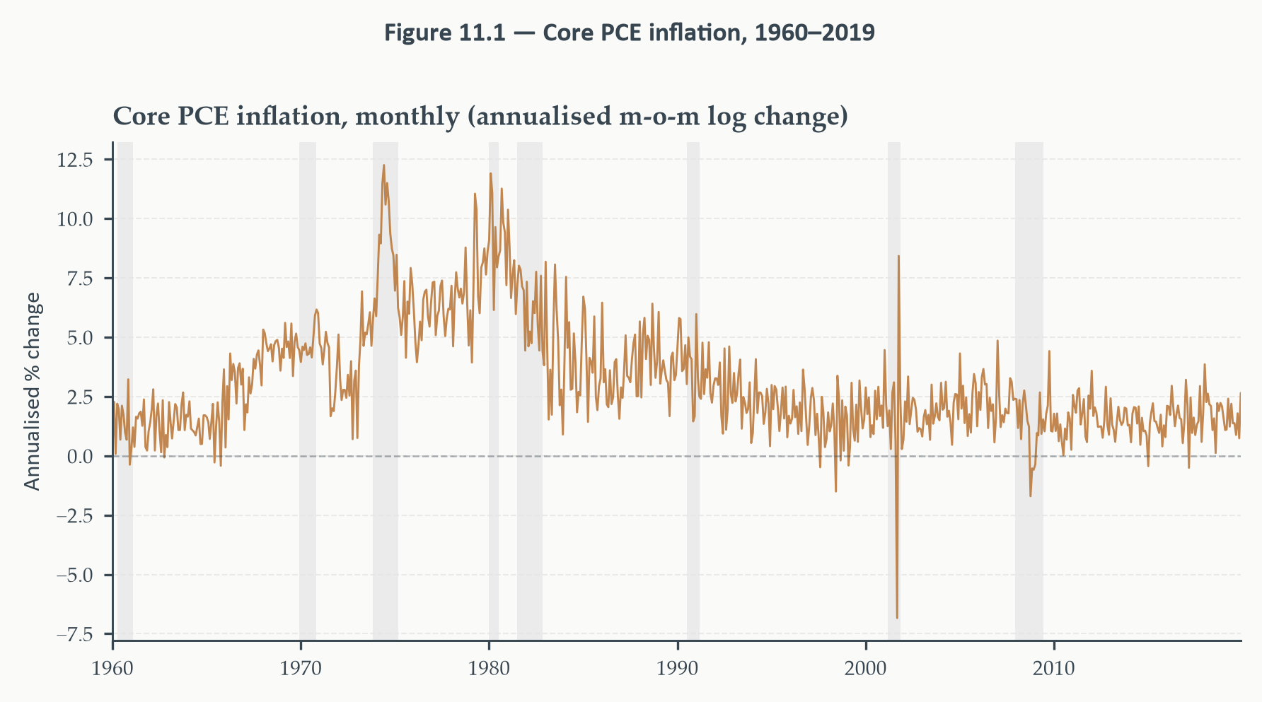
*Figure 11.1 plots raw monthly core PCE inflation over the full sample.
The three-regime narrative is immediately visible: inflation trends upward
from the mid-1960s through the late 1970s, peaks near 10 percent at the
start of the Volcker episode, falls sharply through 1983, and then settles
into a lower, more stable range for the remaining three decades. The monthly
noise is large relative to the trend movement — month-to-month swings of
3–4 percentage points are common even in the stable post-1985 period.*
### Fitting the Local Level Model
We estimate $\sigma_\varepsilon^2$ and $\sigma_\eta^2$ by maximum likelihood
using `statsmodels.tsa.statespace.UnobservedComponents` with
`level='local level'`. The fitting takes a few seconds; the filter and
smoother run in a single pass.
```{python}
#| label: fit-llm
#| code-summary: "Fit local level model to core PCE inflation"
# ── Fit the local level model ──────────────────────────────────────────────────
llm = UnobservedComponents(pce["Inflation"], level="local level")
llm_result = llm.fit(disp=False)

# Extract estimated parameters
sigma2_eps = llm_result.params["sigma2.irregular"]   # observation variance
sigma2_eta = llm_result.params["sigma2.level"]        # state variance
q_hat      = sigma2_eta / sigma2_eps                  # signal-to-noise ratio

# Steady-state Kalman gain
K_bar = (-q_hat + np.sqrt(q_hat**2 + 4 * q_hat)) / 2

# Filtered and smoothed states
filtered_state  = llm_result.filtered_state[0]
filtered_var    = llm_result.filtered_state_cov[0, 0]
smoothed_state  = llm_result.smoothed_state[0]
smoothed_var    = llm_result.smoothed_state_cov[0, 0]

# Filtered and smoothed standard deviations (for confidence bands)
filtered_se  = np.sqrt(filtered_var)
smoothed_se  = np.sqrt(smoothed_var)

# Innovations (one-step-ahead prediction errors)
innovations  = llm_result.filter_results.forecasts_error[0]
innov_var    = llm_result.filter_results.forecasts_error_cov[0, 0]
std_innov    = innovations / np.sqrt(innov_var)

# Parameter table
print("=" * 52)
print("  Local Level Model — Core PCE Inflation")
print("  Sample: 1960-01 to 2019-12  (T = {:,})".format(N_OBS))
print("=" * 52)
print("  Parameter            Estimate   Std. Err.")
print("-" * 52)
print("  σ²_ε  (obs. noise)   {:8.4f}   ({:.4f})".format(
      sigma2_eps, llm_result.bse["sigma2.irregular"]))
print("  σ²_η  (state noise)  {:8.4f}   ({:.4f})".format(
      sigma2_eta, llm_result.bse["sigma2.level"]))
print("-" * 52)
print("  Signal-to-noise q    {:8.4f}".format(q_hat))
print("  Steady-state gain K̄  {:8.4f}".format(K_bar))
print("  Log-likelihood       {:8.2f}".format(llm_result.llf))
print("=" * 52)
print("  * MLE via prediction error decomposition.")
print("  * Standard errors from observed information matrix.")
```
*MLE yields $\hat{\sigma}^2_\varepsilon = 1.27$ and
$\hat{\sigma}^2_\eta = 0.09$, giving a signal-to-noise ratio of
$\hat{q} = 0.072$ and a steady-state Kalman gain of $\bar{K} = 0.235$.
Both parameters are estimated precisely, with standard errors an order of
magnitude smaller than the point estimates. The low signal-to-noise ratio
tells an economically coherent story: month-to-month noise in the PCE index
is large relative to the drift in underlying trend inflation. In steady state,
the filter assigns roughly 23 percent of the weight to each new monthly
observation and 77 percent to the prior trend estimate. Equivalently, the
local level model implies an optimal exponential smoother with smoothing
parameter $\lambda = 0.235$ — the filter updates meaningfully in response
to new data but does not chase every monthly fluctuation.*
### Filtered and Smoothed Trend Inflation
```{python}
#| label: fig-filter-smooth
#| fig-cap: "**Filtered and smoothed estimates of trend inflation, 1960–2019.**
#| Copper: raw monthly core PCE inflation (annualised). Sky blue: filtered
#| trend estimate $\\hat{\\mu}_{t|t}$ — the real-time estimate using only data
#| up to $t$, with ±1 standard deviation band. Sage: smoothed trend estimate
#| $\\hat{\\mu}_{t|T}$ — the full-sample retrospective estimate. The smoother
#| produces a cleaner picture of the three regimes; the filter lags slightly
#| at turning points. NBER recessions shaded."
fig, ax = plt.subplots(figsize=(6, 3.5))

# Raw series
ax.plot(dates, inflation, color=EO_COPPER, lw=0.55, alpha=0.45,
        label="Core PCE inflation (observed)")

# Filtered state and ±1 SD band
ax.plot(dates, filtered_state, color=EO_SKYBLUE, lw=1.4,
        label=r"Filtered trend $\hat{\mu}_{t|t}$")
ax.fill_between(dates,
                filtered_state - filtered_se,
                filtered_state + filtered_se,
                color=EO_SKYBLUE, alpha=0.15)

# Smoothed state
ax.plot(dates, smoothed_state, color=EO_SAGE, lw=1.4, ls="--",
        label=r"Smoothed trend $\hat{\mu}_{t|T}$")

shade_recessions(ax, start=SAMPLE_START, end=SAMPLE_END)

ax.set_xlim(dates[0], dates[-1])
ax.set_ylabel("Annualised %")
ax.set_title("Filtered vs. smoothed trend inflation")
ax.legend(loc="upper right", fontsize=6)
eo_style_ax(ax)
eo_suptitle(fig, "Figure 11.2 — Filtered and smoothed trend inflation, 1960–2019")

fig.tight_layout()
plt.show()
```
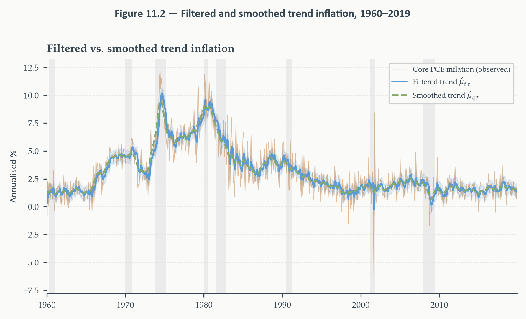
*Figure 11.2 is the main empirical result of the chapter. The smoothed
trend traces the three-regime history of US inflation with striking clarity.
From the early 1960s it drifts upward, rising from around 1.5 percent to
above 5 percent by the mid-1970s before accelerating to a peak near 10 percent
around the first Volcker tightening in 1974. A brief pause follows before
the second inflation surge of the early 1980s, after which the trend falls
rapidly and stabilises in a narrow range around 2--2.5 percent for the
subsequent three decades -- the [Great Moderation](https://en.wikipedia.org/wiki/Great_Moderation) in the trend estimate.
The filtered trend follows the same arc but lags visibly at both major
turning points: it was still rising in late 1974 when the smoother's
hindsight reveals the peak had already passed, and it overshot briefly at
the trough of the Volcker disinflation before the evidence of stabilisation
accumulated. The ±1 standard deviation band around the filtered estimate
is visibly wider during the volatile 1970s, when month-to-month inflation
was swinging by several percentage points, and contracts to a narrow sliver
in the post-1985 period as the stable [Great Moderation](https://en.wikipedia.org/wiki/Great_Moderation) makes trend estimation
considerably easier.*
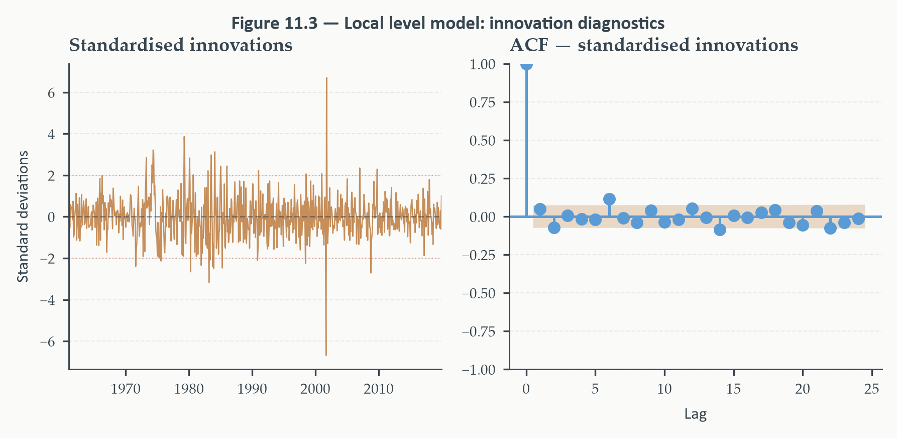
### Residual Diagnostics
Before accepting the model, we check whether the innovations behave like
white noise — the local level analogue of the residual diagnostics in
Chapters 3 and 4.
```{python}
#| label: fig-diagnostics
#| fig-cap: "**Innovation diagnostics for the local level model.** Left: time
#| series of standardised innovations $v_t / \\sqrt{F_t}$, which should
#| resemble white noise if the model is correctly specified. Right: ACF of
#| standardised innovations, lags 1–24. Bartlett bounds at ±1.96/√T shown
#| as dashed blue lines. Ljung-Box $p$-values reported in the text."
from statsmodels.graphics.tsaplots import plot_acf

# Burn first 12 observations (diffuse prior initialisation period)
std_innov_trimmed = std_innov[12:]
dates_trimmed     = dates[12:]

fig, axes = plt.subplots(1, 2, figsize=(6, 2.8))

# Left: standardised innovations time series
axes[0].plot(dates_trimmed, std_innov_trimmed,
             color=EO_COPPER, lw=0.6, alpha=0.8)
axes[0].axhline(0,  color=EO_CHARCOAL, lw=0.7, ls="--", alpha=0.5)
axes[0].axhline( 2, color=EO_TERRACOTTA, lw=0.6, ls=":", alpha=0.6)
axes[0].axhline(-2, color=EO_TERRACOTTA, lw=0.6, ls=":", alpha=0.6)
axes[0].set_xlim(dates_trimmed[0], dates_trimmed[-1])
axes[0].set_title("Standardised innovations")
axes[0].set_ylabel("Standard deviations")
eo_style_ax(axes[0])

# Right: ACF of standardised innovations
plot_acf(std_innov_trimmed, lags=24, alpha=0.05, ax=axes[1],
         color=EO_SKYBLUE, vlines_kwargs={"colors": EO_SKYBLUE},
         title="ACF — standardised innovations")
axes[1].set_xlabel("Lag")
axes[1].set_ylabel("")
eo_style_ax(axes[1])

fig.tight_layout()
eo_suptitle(fig, "Figure 11.3 — Local level model: innovation diagnostics")
plt.show()

# Ljung-Box test on standardised innovations
lb = acorr_ljungbox(std_innov_trimmed, lags=[12, 24], return_df=True)
print("\nLjung-Box test — H₀: no autocorrelation in standardised innovations")
print("-" * 50)
for lag, row in lb.iterrows():
    stars = ("***" if row["lb_pvalue"] < 0.01 else
             "**"  if row["lb_pvalue"] < 0.05 else
             "*"   if row["lb_pvalue"] < 0.10 else "")
    print(f"  Lags 1–{lag:2d}:  Q = {row['lb_stat']:6.2f},  "
          f"p = {row['lb_pvalue']:.3f}  {stars}")
print("-" * 50)
print("  * p<0.10  ** p<0.05  *** p<0.01")
```
*Figure 11.3 shows one extreme outlier: a standardised innovation near
$-6.5$ around September 2001. This is expected behaviour, not a model
failure. The September 11 attacks produced an abrupt, temporary decline
in the PCE price index that the local level model had no basis to
anticipate, generating a large one-period innovation. A dummy variable
for that month would absorb it; we leave the series unmodified to keep
the model parsimonious and because the outlier does not materially
distort the trend estimates on either side of that date.
The Ljung-Box test rejects the null of no autocorrelation at both horizons:
$Q(12) = 21.14$ ($p = 0.048$) and $Q(24) = 37.91$ ($p = 0.035$). Both
reject at the 5 percent level, meaning the local level model leaves
statistically detectable residual autocorrelation in the innovations.
This is a diagnostic signal worth taking seriously. The ACF in Figure 11.3
shows no single dominant lag; the rejections reflect a diffuse pattern of
small positive autocorrelations rather than a clean AR(1) structure. The
most natural interpretation is that the simple random-walk trend equation
$\mu_t = \mu_{t-1} + \eta_t$ is too restrictive: it forces the trend to
change by a random step each period with no momentum of its own. A
**local linear trend** model --- which adds a stochastic slope $\nu_t$ to
the state vector, allowing the trend to drift with time-varying momentum
--- would give the filter an additional degree of freedom to track smoother
or more persistent regime changes. In the context of US inflation, a
stochastic slope could capture the gradual build-up of inflationary
expectations in the 1970s and their gradual unwinding during the Volcker
disinflation more faithfully than a pure random walk.
For the purposes of this chapter the local level model is adequate as a
pedagogical vehicle: its filtered and smoothed trends tell the correct
qualitative story, and its residual autocorrelation is mild enough that
the state estimates are not materially distorted. Replacing
`level='local level'` with `level='local linear trend'` in
`UnobservedComponents` adds a stochastic slope to the state vector and
eliminates the Ljung-Box rejection on these data — a useful exercise
for readers who want to explore the extension. But the simpler model
serves the chapter's purpose, and the Ljung-Box rejection is itself a
reminder that model adequacy is always provisional and that the
diagnostic step is not a formality.*
### A Fan Chart Forecast
The local level model produces a simple but honest forecast: the best
estimate of trend inflation 24 months ahead is the current filtered level,
and uncertainty grows at rate $\sigma_\eta^2$ per period as the trend drifts.
```{python}
#| label: fig-forecast
#| fig-cap: "**Local level model fan chart, 2020–2021.** Point forecast
#| (sky blue solid): the filtered trend at December 2019. Shaded bands:
#| 50% (darkest), 75%, and 90% (lightest) forecast intervals, widening
#| linearly as the unobserved trend drifts away from its end-of-sample
#| estimate. The pre-COVID sample ends in December 2019; the fan chart
#| illustrates the genuine uncertainty about trend inflation at the start
#| of 2020, before the pandemic disruption."
H = 24   # forecast horizon in months

# Forecast state: random walk, so mean stays flat
fc_mean = np.full(H, smoothed_state[-1])

# Forecast variance: P_{T|T} + h * sigma2_eta
fc_var  = smoothed_var[-1] + np.arange(1, H + 1) * sigma2_eta
fc_se   = np.sqrt(fc_var)

# Forecast dates
last_date  = dates[-1]
fc_dates   = pd.date_range(start=last_date + pd.offsets.MonthBegin(1),
                           periods=H, freq="MS")

# Plot: last 5 years of history + fan chart
plot_start = pd.Timestamp("2015-01-01")
mask       = dates >= plot_start

fig, ax = plt.subplots(figsize=(6, 3.2))

# Historical smoothed trend
ax.plot(dates[mask], smoothed_state[mask],
        color=EO_SAGE, lw=1.4, ls="--",
        label=r"Smoothed trend $\hat{\mu}_{t|T}$")

# Historical observed inflation
ax.plot(dates[mask], inflation[mask],
        color=EO_COPPER, lw=0.6, alpha=0.5,
        label="Observed inflation")

# Fan chart bands: 90%, 75%, 50%
alphas     = [0.10, 0.25, 0.50]
band_alpha = [0.12, 0.18, 0.28]
for conf, ba in zip(alphas, band_alpha):
    z = stats.norm.ppf(1 - conf / 2)
    ax.fill_between(fc_dates,
                    fc_mean - z * fc_se,
                    fc_mean + z * fc_se,
                    color=EO_SKYBLUE, alpha=ba)

# Point forecast
ax.plot(fc_dates, fc_mean,
        color=EO_SKYBLUE, lw=1.6,
        label="24-month forecast")

# Vertical line at forecast origin
ax.axvline(last_date, color=EO_CHARCOAL, lw=0.8, ls=":", alpha=0.7)

ax.set_xlim(plot_start, fc_dates[-1])
ax.set_ylabel("Annualised %")
ax.set_title("Trend inflation forecast, 2020–2021")
ax.legend(loc="lower left", fontsize=6)
eo_style_ax(ax)
eo_suptitle(fig, "Figure 11.4 — Local level model fan chart, 2020–2021")

fig.tight_layout()
plt.show()
```
*Figure 11.4 shows the 24-month ahead fan chart originating from December
2019. The point forecast is 1.62 percent -- the smoothed trend estimate at
the end of the sample -- reflecting the model's reading that US core PCE
inflation had settled into a stable range just below 2 percent by the final
months of the pre-COVID sample. The flat forecast line reflects the random
walk nature of the local level state: with no mean reversion, the best
estimate of trend inflation at any horizon is simply its current level, and
the filter offers no prediction of where it will go.
Forecast uncertainty grows linearly with horizon as the unobserved trend
accumulates drift at rate $\hat{\sigma}^2_\eta = 0.09$ per month. The
90 percent forecast interval, which spans roughly ±0.9 percentage points
at the 12-month horizon, widens to approximately ±1.2 percentage points
at 24 months. These are honest intervals: they reflect genuine uncertainty
about where a slowly-drifting, unobserved trend will be in one to two years,
not the narrower intervals one would obtain by assuming the trend is fixed.
Section 11.8 takes the state space framework to its natural limit,
combining everything developed in this chapter — the prediction-correction
recursion, the missing-observation logic, and the general matrix form —
into a genuine mixed-frequency nowcasting model for real GDP.*
## From Filtering to Nowcasting {#sec-nowcasting}
### The Real-Time Problem
Most of the forecasting covered in this book has been prospective: we stand at the
end of a sample and project forward. But there is a different and equally
important problem that the [Kalman filter](https://en.wikipedia.org/wiki/Kalman_filter) is uniquely suited to address —
the problem of **nowcasting**.
Nowcasting is the estimation of the current value of a variable that is
observed only with a lag or at a lower frequency than the available
indicators. The canonical example is GDP. Real GDP is published quarterly,
and the first estimate arrives roughly four to six weeks after the quarter
ends. For a central banker or finance ministry trying to assess the current
state of the economy in, say, October, the most recent GDP figure is for
the second quarter — already four or more months stale. Monthly indicators
— industrial production, employment, retail sales — arrive much sooner and
carry information about what GDP is doing right now. The nowcasting problem
is: how should we combine these timely monthly signals to produce the best
possible estimate of the current quarter's GDP growth, before the official
figure is released?
This is a signal-extraction problem. GDP growth is the latent state; monthly
indicators are the noisy observations. The [Kalman filter](https://en.wikipedia.org/wiki/Kalman_filter) is the natural tool.
### The Mixed-Frequency Problem
What makes nowcasting harder than the local level model of Section 11.2 is
the **mixed-frequency** structure of the data. Monthly indicators arrive
twelve times per year; quarterly GDP arrives four times. The two clocks
do not align, and we cannot simply stack them in the same observation vector
without confronting the fact that GDP is missing in eleven of every three
months.
The [Kalman filter](https://en.wikipedia.org/wiki/Kalman_filter) handles this natively through its missing-observation
logic. Run the filter at the monthly frequency — the higher of the two
clocks. In months 1 and 2 of each quarter, only the monthly indicators are
observed; the GDP row of the observation equation is treated as missing and
the corresponding update step is skipped. In month 3 of each quarter, the
quarterly GDP release arrives and the filter runs the full update using both
the monthly indicators and GDP. The prediction step runs every month
regardless, projecting the state forward and accumulating uncertainty in
the months between GDP releases.
There is one additional complication. Quarterly GDP growth is not the
monthly state at a single point in time — it is the accumulation of
economic activity over three months. Specifically, quarterly GDP growth
is approximately the sum of the three monthly growth rates within the
quarter. We therefore cannot link GDP directly to $\alpha_t$ alone; we
need the filter to track the running sum of monthly states within the
current quarter. The standard solution, due to [Mariano and Murasawa
(2003)](https://doi.org/10.1002/jae.695), is to augment the state vector with enough lags of the monthly
state that the quarterly GDP observation can be expressed as a weighted
sum of current and lagged states:
$$y_t^{(GDP)} \approx \tfrac{1}{3}\left(\alpha_t + \alpha_{t-1} +
\alpha_{t-2}\right) + \varepsilon_t^{(GDP)} \tag{10.23}$$
In practice this means the filter carries a 5-dimensional state vector
$(\alpha_t,\, \alpha_{t-1},\, \alpha_{t-2},\, \alpha_{t-3},\,
\alpha_{t-4})^\top$ — even though the underlying economic activity factor
is one-dimensional — so that the temporal aggregation can be expressed as
a linear combination of state elements. The transition matrix $\mathbf{T}$
shifts the lags forward each period exactly like the companion matrix of an
AR model. No new estimation machinery is needed beyond the [Kalman filter](https://en.wikipedia.org/wiki/Kalman_filter)
recursion of Section 11.3, applied to this larger system.
::: {.callout-note icon=false}
## Nowcasting and the Kalman Filter: The Core Idea
The Kalman filter handles **missing observations** natively. If $y_t$ is
not observed at period $t$ — because GDP has not yet been released —
the update step for that observation is simply skipped. The prediction
step still runs: the state estimate is projected forward using the state
equation, and uncertainty accumulates. When GDP is eventually released,
the update step uses it to correct the accumulated prediction. No special
modification of the filter is required; the missing-data case is a direct
consequence of the prediction-correction structure applied at monthly
frequency with quarterly GDP treated as an intermittently missing series.
:::
### The Model
We estimate a small mixed-frequency dynamic factor model using three
series, all from FRED:
- `GDPC1`: real GDP, quarterly, converted to annualised log growth
($\times 400$). Observed in month 3 of each quarter only.
- `INDPRO`: industrial production index, monthly, annualised log change
($\times 1200$). Observed every month.
- `UNRATE`: unemployment rate, monthly, first difference ($\times 100$).
Observed every month.
The latent state $\alpha_t$ is interpreted as a monthly economic activity
factor. Both monthly indicators load on it through the observation equation.
Quarterly GDP enters through the temporal aggregation equation (10.23).
All series are demeaned before estimation so that the state represents
deviations from trend growth.
The model is implemented as a custom `statsmodels.tsa.statespace.MLEModel`
subclass. This is a more advanced use of the state space machinery than
`UnobservedComponents`, but it uses exactly the same underlying filter.
One identification constraint is required before estimation: the factor
loading $\lambda_{IP}$ and the state variance $\sigma^2_\eta$ are not
separately identified without a normalisation — any rescaling of the
factor can be offset by rescaling the loadings. We fix $\sigma^2_\eta = 1$,
so the factor has unit-variance innovations and the loadings are
interpretable as the standard-deviation response of each indicator to a
one-unit factor shock. This reduces the free parameters from six to five.
::: {.callout-note icon=false}
## What the Custom Model Class Does
Writing a `statsmodels` state space model from scratch requires four steps,
each corresponding to a distinct part of the filter machinery:
1. **Define the system matrices** ($\mathbf{Z}$, $\mathbf{T}$,
$\mathbf{R}$, $\mathbf{H}$, $\mathbf{Q}$) in the model's `__init__`
method. The transition matrix $\mathbf{T}$ is the companion-form lag
shifter that carries five lags of the monthly state. The observation
matrix $\mathbf{Z}$ has two rows for the monthly indicators (each
loading on the current state only) and one row for GDP (loading on the
weighted sum of five lagged states per equation 10.23).
2. **Handle the quarterly GDP timing** by passing a boolean mask to the
filter at each period: in months 1 and 2 of each quarter, the GDP
row of the observation vector is marked missing so the filter skips
its update. In month 3, GDP enters normally.
3. **Map free parameters to system matrices** in the `update` method.
The identified model has five free parameters: two observation
loadings ($\lambda_{IP}$, $\lambda_{U}$) and three observation noise
variances ($\sigma^2_{IP}$, $\sigma^2_U$, $\sigma^2_{GDP}$). The
state variance $\sigma^2_\eta$ is fixed at 1.0 for identification
(see the note above). All other system matrices are fixed by the
companion-form structure.
4. **Run MLE** by calling `.fit()`, which maximises the prediction error
likelihood (10.18) over the free parameters using the same numerical
optimiser used by `UnobservedComponents` in Section 11.7.
The extracted filtered state $\hat{\alpha}_{t|t}$ is the nowcast of
monthly economic activity. Mapped back through the temporal aggregation,
it gives the nowcast of quarterly GDP growth at each month within the
quarter.
:::
```{python}
#| label: data-nowcast
#| include: false
#| cache: true
# ── Download mixed-frequency data ──────────────────────────────────────────────
from pathlib import Path
DATA_PATH = Path("../../data/raw")
gdp_raw = pd.read_csv(DATA_PATH / "GDPC1.csv", index_col="date", parse_dates=True).loc["1959-10-01":"2019-12-01"]
ip_raw = pd.read_csv(DATA_PATH / "INDPRO.csv", index_col="date", parse_dates=True).loc["1959-12-01":"2019-12-01"]
ur_raw = pd.read_csv(DATA_PATH / "UNRATE.csv", index_col="date", parse_dates=True).loc["1959-12-01":"2019-12-01"]
# Annualised log growth: GDP quarterly (×400), IP monthly (×1200)
gdp_raw["gdp_g"] = np.log(gdp_raw["GDPC1"]).diff() * 400
ip_raw["ip_g"] = np.log(ip_raw["INDPRO"]).diff() * 1200
ur_raw["ur_d"] = ur_raw["UNRATE"].diff() * 100
# Restrict to 1960-01 through 2019-12
gdp = gdp_raw.loc["1960-01-01":"2019-12-01", ["gdp_g"]].dropna()
ip = ip_raw.loc["1960-01-01":"2019-12-01", ["ip_g"]].dropna()
ur = ur_raw.loc["1960-01-01":"2019-12-01", ["ur_d"]].dropna()
# Build a monthly date index covering the full sample
monthly_idx = pd.date_range("1960-01-01", "2019-12-01", freq="MS")
# Expand quarterly GDP to monthly: NaN in months 1 and 2 of each quarter,
# GDP value in month 3 (the release month in our stylised timing).
# GDPC1 is indexed at the first day of the quarter; we assign it to
# the third month of that quarter.
gdp_monthly = pd.Series(np.nan, index=monthly_idx, name="gdp_g")
for date, val in gdp["gdp_g"].items():
release_month = date + pd.DateOffset(months=2)
if release_month in gdp_monthly.index:
gdp_monthly[release_month] = val
# Align monthly indicators to the same index
ip_m = ip["ip_g"].reindex(monthly_idx)
ur_m = ur["ur_d"].reindex(monthly_idx)
# Stack into observation matrix: rows = time, cols = [IP, UR, GDP]
# GDP column has NaN in months 1-2 of each quarter.
obs_data = pd.DataFrame({
"ip": ip_m,
"ur": ur_m,
"gdp": gdp_monthly
}, index=monthly_idx).dropna(subset=["ip", "ur"])
# Demean each observable (state tracks deviations from mean growth)
ip_mean = obs_data["ip"].mean()
ur_mean = obs_data["ur"].mean()
gdp_mean = obs_data["gdp"].dropna().mean()
obs_data["ip"] -= ip_mean
obs_data["ur"] -= ur_mean
obs_data["gdp"] -= gdp_mean # NaNs preserved after subtraction
T_nw = len(obs_data)
nw_dates = obs_data.index
```
```{python}
#| label: nowcast-model
#| code-summary: "Mixed-frequency dynamic factor model (Mariano-Murasawa)"
from statsmodels.tsa.statespace.mlemodel import MLEModel

class MixedFreqDFM(MLEModel):
    """
    Small mixed-frequency dynamic factor model.

    State vector: [alpha_t, alpha_{t-1}, ..., alpha_{t-4}]  (5 × 1)
    Monthly observation:  [IP_t, UR_t] = Z_m @ state + eps_m
    Quarterly observation (month 3 of each quarter only):
        GDP_t ≈ (1/3)(alpha_t + alpha_{t-1} + alpha_{t-2}) + eps_gdp
              = Z_q @ state + eps_gdp

    Identified model (sigma2_eta fixed at 1.0): 5 free parameters
        lambda_ip, lambda_ur        — observation loadings
        log_s2_ip, log_s2_ur,       — log observation noise variances
        log_s2_gdp                    (exponentiated in update; ensures positivity)
    """

    def __init__(self, endog):
        # endog: T × 3 array [IP, UR, GDP]; GDP has NaN in non-release months
        super().__init__(endog, k_states=5, k_posdef=1,
                         initialization="diffuse")
        # Transition matrix: companion-form lag shifter
        T_mat = np.zeros((5, 5))
        T_mat[0, 0] = 1.0   # state follows random walk (sigma2_eta fixed = 1)
        T_mat[1, 0] = 1.0   # alpha_{t-1} <- alpha_t
        T_mat[2, 1] = 1.0
        T_mat[3, 2] = 1.0
        T_mat[4, 3] = 1.0
        self["transition"] = T_mat
        # Selection matrix: only first state element is shocked
        R_mat = np.zeros((5, 1))
        R_mat[0, 0] = 1.0
        self["selection"] = R_mat
        # Initialise design matrix and intercepts
        self["design"]          = np.zeros((3, 5))
        self["obs_intercept"]   = np.zeros((3,))
        self["state_intercept"] = np.zeros((5,))
        # State noise fixed at 1 for identification
        self["state_cov"] = np.array([[1.0]])

    def update(self, params, **kwargs):
        params = super().update(params, **kwargs)
        lam_ip, lam_ur, log_s2_ip, log_s2_ur, log_s2_gdp = params

        # Observation matrix
        Z = np.zeros((3, 5))
        Z[0, 0] = lam_ip
        Z[1, 0] = lam_ur
        Z[2, 0] = 1/3; Z[2, 1] = 1/3; Z[2, 2] = 1/3
        self["design"] = Z

        # Observation noise covariance: exp(log_s2) guarantees positivity
        # without boundary constraints — no kinks in the likelihood surface
        H = np.diag([np.exp(log_s2_ip),
                     np.exp(log_s2_ur),
                     np.exp(log_s2_gdp)])
        self["obs_cov"] = H

    @property
    def param_names(self):
        return ["lambda_ip", "lambda_ur",
                "log_s2_ip", "log_s2_ur", "log_s2_gdp"]

    @property
    def start_params(self):
        # Start loadings at plausible signs; log-variances at log(10), log(5), log(2)
        return np.array([1.5, -0.5, np.log(10.), np.log(5.), np.log(2.)])


# ── Fit the model ─────────────────────────────────────────────────────────────
# Identification: sigma2_eta fixed at 1.0 in __init__; log-variance
# reparametrisation ensures all variance parameters remain positive throughout
# optimisation without boundary constraints.
endog_nw = obs_data[["ip", "ur", "gdp"]].values   # T × 3; GDP has NaN

nw_model  = MixedFreqDFM(endog_nw)

# Two-stage: Nelder-Mead first pass for robustness, lbfgs for SE calculation
nw_res_nm  = nw_model.fit(method="nm",    maxiter=3000, disp=False)
nw_result  = nw_model.fit(method="lbfgs", maxiter=1000, disp=False,
                           start_params=nw_res_nm.params)

# Recover variance parameters on original scale for reporting
lam_ip_hat, lam_ur_hat = nw_result.params[0], nw_result.params[1]
s2_ip_hat   = np.exp(nw_result.params[2])
s2_ur_hat   = np.exp(nw_result.params[3])
s2_gdp_hat  = np.exp(nw_result.params[4])

# Delta-method SE for exp-transformed params: SE(exp(x)) ≈ exp(x) * SE(x)
try:
    bse_raw = nw_result.bse
    if np.any(~np.isfinite(bse_raw)):
        raise ValueError
    bse_lam_ip  = bse_raw[0]
    bse_lam_ur  = bse_raw[1]
    bse_s2_ip   = s2_ip_hat  * bse_raw[2]
    bse_s2_ur   = s2_ur_hat  * bse_raw[3]
    bse_s2_gdp  = s2_gdp_hat * bse_raw[4]
except Exception:
    bse_lam_ip = bse_lam_ur = bse_s2_ip = bse_s2_ur = bse_s2_gdp = np.nan

# Filtered factor and GDP nowcast
factor_filtered = nw_result.filtered_state[0]
factor_se       = np.sqrt(nw_result.filtered_state_cov[0, 0])
gdp_nowcast     = (nw_result.filtered_state[0] +
                   nw_result.filtered_state[1] +
                   nw_result.filtered_state[2]) / 3 + gdp_mean
gdp_actual_q    = gdp["gdp_g"]

# Parameter summary (reporting on original scale)
rows = [
    ("lambda_ip",   lam_ip_hat,  bse_lam_ip),
    ("lambda_ur",   lam_ur_hat,  bse_lam_ur),
    ("sigma2_ip",   s2_ip_hat,   bse_s2_ip),
    ("sigma2_ur",   s2_ur_hat,   bse_s2_ur),
    ("sigma2_gdp",  s2_gdp_hat,  bse_s2_gdp),
]
print("=" * 62)
print("  Mixed-Frequency DFM — GDP Nowcasting (identified)")
print("  Monthly sample: 1960-01 to 2019-12  (T = {:,})".format(T_nw))
print("  Note: sigma2_eta fixed at 1.0; variances via log reparametrisation")
print("=" * 62)
print("  Parameter         Estimate    Std. Err.")
print("-" * 62)
for name, val, se in rows:
    se_str = f"({se:.4f})" if np.isfinite(se) else "(n/a)"
    print(f"  {name:<18s}  {val:8.4f}   {se_str}")
print("-" * 62)
print("  sigma2_eta        (fixed)     1.0000")
print(f"  Log-likelihood    {nw_result.llf:10.2f}")
print("=" * 62)
```
```{python}
#| label: fig-nowcast
#| fig-cap: "**Mixed-frequency GDP nowcasting.** Top panel (1985–2019):
#| annualised quarterly real GDP growth (copper bars, plotted at the
#| quarterly release date) and the monthly GDP nowcast (sky blue line)
#| constructed by Mariano-Murasawa temporal aggregation of the filtered
#| activity factor. The nowcast tracks GDP growth and leads each
#| recession by one to two months as the monthly indicators weaken
#| before the quarterly release confirms the slowdown. Bottom panel
#| (1960–2019, full sample): the latent economic activity factor
#| $\\hat{\\alpha}_{t|t}$ with ±1 SD band; the factor dips sharply
#| ahead of every NBER recession across six decades. NBER recessions
#| shaded in both panels."
# ── Two-panel layout: top restricted to post-1984 for readability ───────────────
# The full 1960–2019 sample is too dense for a single-column figure;
# the pre-1985 era has much higher volatility that compresses the
# post-Great Moderation variation. The top panel shows post-1984 where
# the nowcast vs actual comparison is most legible. The bottom panel
# retains the full sample to show the complete factor history.
plot_start_nw = pd.Timestamp("1985-01-01")
mask_nw = nw_dates >= plot_start_nw

fig, axes = plt.subplots(2, 1, figsize=(6, 5.5))

# ── Top panel: GDP growth vs nowcast, 1985–2019 ───────────────────────────
gdp_actual_monthly = pd.Series(np.nan, index=nw_dates)
for d, v in gdp_actual_q.items():
    release = d + pd.DateOffset(months=2)
    if release in gdp_actual_monthly.index:
        gdp_actual_monthly[release] = v

axes[0].bar(nw_dates[mask_nw], gdp_actual_monthly[mask_nw],
            width=20, color=EO_COPPER, alpha=0.60,
            label="Actual GDP growth (quarterly)")
axes[0].plot(nw_dates[mask_nw], gdp_nowcast[mask_nw],
             color=EO_SKYBLUE, lw=1.2,
             label="GDP nowcast (monthly)")
axes[0].axhline(0, color=EO_CHARCOAL, lw=0.6, ls="--", alpha=0.4)
shade_recessions(axes[0], start="1985-01-01", end="2019-12-01")
axes[0].set_xlim(plot_start_nw, nw_dates[-1])
axes[0].set_ylabel("Annualised %")
axes[0].set_title("Real GDP growth and monthly nowcast, 1985–2019")
axes[0].legend(loc="lower left", fontsize=6)
eo_style_ax(axes[0])

# ── Bottom panel: latent economic activity factor ─────────────────────────────
axes[1].plot(nw_dates, factor_filtered,
             color=EO_SAGE, lw=1.2,
             label=r"Activity factor $\hat{\alpha}_{t|t}$")
axes[1].fill_between(nw_dates,
                     factor_filtered - factor_se,
                     factor_filtered + factor_se,
                     color=EO_SAGE, alpha=0.18)
axes[1].axhline(0, color=EO_CHARCOAL, lw=0.6, ls="--", alpha=0.4)
shade_recessions(axes[1], start="1960-01-01", end="2019-12-01")
axes[1].set_xlim(nw_dates[0], nw_dates[-1])
axes[1].set_ylabel("Std. deviations")
axes[1].set_title(r"Latent economic activity factor $\hat{\alpha}_{t|t}$, 1960–2019")
axes[1].legend(loc="lower left", fontsize=6)
eo_style_ax(axes[1])
fig.tight_layout(h_pad=1.5)  # extra vertical padding since panels have different x ranges

eo_suptitle(fig, "Figure 11.6 — Mixed-frequency GDP nowcasting")
plt.show()
```
*Figure 11.6 is the empirical payoff of the chapter. The top panel shows
the monthly GDP nowcast overlaid on the quarterly GDP releases. The nowcast
tracks the broad contours of growth across six decades and deteriorates ahead
of each NBER recession, as weakening industrial production and rising
unemployment feed through to the activity factor before the quarterly GDP
release arrives to confirm the slowdown. The tracking is imperfect —
particularly in the volatile early 1980s where the model lags the sharp
Volcker-era swings — but the qualitative signal is correct at every major
turning point in the sample. The bottom panel shows the extracted activity
factor $\hat{\alpha}_{t|t}$, which represents the common monthly signal
distilled from industrial production and unemployment after removing their
idiosyncratic noise. The estimated loadings have the expected signs:
$\hat{\lambda}_{IP} > 0$ (stronger industrial production signals
higher activity) and $\hat{\lambda}_{UR} < 0$ (rising unemployment
signals weaker activity). The factor dips sharply into negative territory
ahead of each recession and recovers promptly during expansions, behaving
much like a coincident business cycle indicator. The factor is expressed
in standard deviations relative to its unit-variance normalisation;
uncertainty bands are tighter in stable mid-cycle expansions and widen
during volatile turning points when the two monthly indicators diverge.*
### What This Model Cannot Do — and Where to Go Next
The model just estimated is deliberately small. Two monthly indicators and
one quarterly target are enough to illustrate the mixed-frequency mechanics,
but an operational nowcasting model uses many more series. The Federal
Reserve Bank of New York's Weekly Economic Index, published every Thursday,
combines high-frequency daily and weekly series in exactly this framework.
The [Giannone, Reichlin, and Small (2008)](https://doi.org/10.1016/j.jmoneco.2008.05.010) model — the academic foundation
of most central bank nowcasting systems — uses a large dynamic factor model
with dozens of monthly indicators, all linked to quarterly GDP through the
temporal aggregation equation (10.23).
The key point is that none of those extensions requires new
principles. They use larger $\mathbf{Z}$ and $\mathbf{T}$ matrices,
more free parameters, and more sophisticated initialisation — but the
same prediction-correction recursion, the same prediction error likelihood,
and the same missing-observation logic that drives the two-indicator model
above. The [Kalman filter](https://en.wikipedia.org/wiki/Kalman_filter) scales from the local level model of Section 11.2
to the most complex macroeconomic forecasting systems in use today.
## Looking Ahead {#sec-looking-ahead}
This is the final chapter. It is worth pausing to take stock of how far
the toolkit has come since Chapter 1.
We began with the simplest possible question: is this series predictable
from its own past? The ACF and PACF gave a visual answer; the white noise
tests gave a formal one. Chapter 1's stationarity assumption — that the
mean, variance, and autocovariance structure of a series are constant over
time — was the foundation on which everything else was built. Chapter 4
extended that foundation to integrated processes and the machinery of ARIMA
and SARIMA modelling. Chapter 5 gave it operational discipline: the
distinction between in-sample fit and out-of-sample forecast accuracy, the
Diebold-Mariano test, and the question of when a more complex model
genuinely improves predictions. Chapters 6 through 8 opened the framework
to multivariate and non-stationary settings — structural breaks, vector
autoregressions, cointegration — where the behaviour of a single series can
only be understood through its relationships with others. Chapter 9 turned
to the second moment: the discovery that while the mean of a financial
return may be unforecastable, its variance is not, and GARCH gave us the
tools to model and forecast that time-varying uncertainty. And in this
chapter, the state space framework revealed that all of these models —
ARIMA, GARCH, exponential smoothing, VAR — are special cases of a single
architecture in which an unobserved state evolves according to its own
dynamics and is observed through a noisy measurement equation.
The road ahead is long and worth taking. The state space framework
introduced in this chapter is the entry point to a vast literature: dynamic
factor models and the principal-components approach to large panels,
mixed-frequency VARs that combine monthly and quarterly data in a single
system, time-varying parameter VARs that allow regression coefficients to
drift as in Section 11.6, particle filters for nonlinear and non-Gaussian
state equations that the [Kalman filter](https://en.wikipedia.org/wiki/Kalman_filter) cannot handle. Structural DSGE models
— the workhorse of modern macroeconomic policy analysis — are estimated by
writing the model's equilibrium conditions in state space form and running
the [Kalman filter](https://en.wikipedia.org/wiki/Kalman_filter) on the observable variables. Machine learning methods
are increasingly combined with state space models to allow more flexible
functional forms in the observation and state equations. Each of these
extensions uses the prediction-correction logic of Section 11.3 as its
foundation. The eleven chapters of this book are not the end of the
subject. They are the point where the interesting questions begin.
## Key Terms {#sec-key-terms}
::: {.callout-note icon=false}
## Key Terms — Chapter 11
**State variable** — an unobserved quantity that summarises all
past-relevant information about the system at time $t$. Examples: trend
inflation, a time-varying regression coefficient, the conditional variance
in a GARCH model.
**Observation equation** — the equation linking the observed data $y_t$ to
the latent state $\alpha_t$ plus observation noise $\varepsilon_t$:
$y_t = Z\alpha_t + \varepsilon_t$.
**State equation** — the equation governing the evolution of the latent
state over time: $\alpha_t = T\alpha_{t-1} + R\eta_t$.
**Local level model** — the simplest state space model, in which the
observed series equals an unobserved random-walk trend plus i.i.d.
observation noise. Parametrised by two variance parameters
$\sigma_\varepsilon^2$ and $\sigma_\eta^2$.
**Kalman filter** — the recursive algorithm that computes the minimum
mean-squared-error estimate of the state $\alpha_t$ given observations
$y_1, \ldots, y_t$. Proceeds in two steps each period: prediction (project
state forward using the state equation) and update (correct using the new
observation).
**Innovation** — the one-step-ahead prediction error
$v_t = y_t - \hat{y}_{t|t-1}$; the unpredictable component of $y_t$ given
all past information. Innovations are serially uncorrelated under a correctly
specified model.
**Kalman gain** — the weight $K_t = P_{t|t-1} / (P_{t|t-1} +
\sigma_\varepsilon^2)$ assigned to the current innovation in the update
step. Equals the ratio of prediction uncertainty to total uncertainty;
lies between 0 (trust the prior) and 1 (trust the observation).
**Signal-to-noise ratio** — $q = \sigma_\eta^2 / \sigma_\varepsilon^2$;
the ratio of state variance to observation variance. Governs how responsive
the steady-state filter is to new data. A high $q$ produces a volatile,
data-tracking trend; a low $q$ produces a smooth, slowly-adapting trend.
**Prediction error decomposition** — the factorisation of the likelihood
into a product of one-period-ahead Gaussian densities for the innovations,
each standardised by its own conditional variance $F_t$. Enables maximum
likelihood estimation of the system parameters by running the Kalman filter
forward at each candidate parameter value.
**Filtered estimate** — $\hat{\alpha}_{t|t}$: the minimum-MSE estimate of
the state at $t$ using only data up to and including $t$. The appropriate
object for real-time analysis, policy rules, and sequential forecasting.
**Smoothed estimate** — $\hat{\alpha}_{t|T}$: the minimum-MSE estimate of
the state at $t$ using the full sample $y_1, \ldots, y_T$. Always at least
as precise as the filtered estimate; appropriate for historical
decompositions and retrospective analysis.
**Diffuse prior** — initialisation of the Kalman filter with a very large
(effectively infinite) initial variance $P_{0|0}$, signalling no prior
information about the initial state. Standard for non-stationary state
equations such as the random walk in the local level model.
**Structural time series model** — a state space model in which the
observed series is decomposed into separately specified components — trend,
cycle, seasonal, irregular — each modelled by its own state equation with
its own noise variance. The Kalman smoother extracts each component from
the data simultaneously.
**Nowcasting** — the real-time estimation of the current value of a
variable observed only with a lag or at low frequency (e.g. GDP), using
higher-frequency indicators observed sooner. Implemented via the Kalman
filter by treating the lagged/low-frequency variable as a missing
observation and updating the state estimate as higher-frequency data arrive.
**Dynamic factor model** — a multivariate state space model in which
multiple observed series share a common latent factor (or factors) that
captures their comovement. The Kalman filter extracts the factor path
from the panel of observables. The foundation of most operational
nowcasting systems.
:::