---
title: "Stationary Time Series Models"
author: ""
abstract: |
The models in this chapter are the workhorses of time series econometrics. Starting
from the simple intuition that today's value of a series depends on its own past,
we build the autoregressive, moving average, and ARMA model families from first
principles. The unifying language is the lag polynomial — a compact algebraic
object whose roots determine whether a model is stationary, invertible, and
well-identified. The chapter develops a complete workflow: from the theoretical
structure of each model class, through the Wold decomposition that justifies
the MA representation of any stationary process, to the Box-Jenkins identification
strategy, maximum likelihood estimation, residual diagnostics, and forecasting.
We close with ARMAX models, which extend the framework to include exogenous
regressors. The tools developed here are the foundation for every model class
that follows.
jupyter: python3
format:
html:
toc: true
toc-depth: 3
toc-title: "In this chapter"
number-sections: true
code-fold: true
code-summary: "Show code"
code-tools: true
theme: cosmo
css: styles.css
highlight-style: github
fig-align: center
fig-cap-location: bottom
fig-responsive: true
html-math-method: mathjax
embed-resources: false
execute:
echo: true
warning: false
message: false
cache: false
---
```{python}
#| label: setup
#| include: false
import numpy as np
import pandas as pd
import matplotlib.pyplot as plt
import matplotlib as mpl
import matplotlib.ticker as mticker
from statsmodels.tsa.stattools import adfuller, kpss, acf, pacf
from statsmodels.graphics.tsaplots import plot_acf, plot_pacf
from statsmodels.tsa.arima.model import ARIMA
import pandas_datareader.data as web
from datetime import datetime
import warnings
warnings.filterwarnings("ignore")
# ── EO Brand Palette ───────────────────────────────────────────────────────────
EO_CHARCOAL = "#36454F"
EO_COPPER = "#B87333"
EO_SAGE = "#87A96B"
EO_SKYBLUE = "#5B9BD5"
EO_TERRACOTTA = "#D4745E"
EO_LAVENDER = "#8E7AB5"
EO_COLORS = [EO_COPPER, EO_SKYBLUE, EO_SAGE,
EO_TERRACOTTA, EO_LAVENDER, EO_CHARCOAL]
PAGE_BG = "#FAFAF8"
# ── Global rcParams ────────────────────────────────────────────────────────────
mpl.rcParams.update({
"figure.figsize": (6, 3),
"figure.dpi": 150,
"figure.facecolor": PAGE_BG,
"figure.edgecolor": PAGE_BG,
"axes.facecolor": PAGE_BG,
"axes.edgecolor": EO_CHARCOAL,
"axes.linewidth": 0.7,
"axes.grid": True,
"axes.grid.axis": "y",
"axes.spines.top": False,
"axes.spines.right": False,
"axes.titlesize": 9,
"axes.titleweight": "bold",
"axes.titlecolor": EO_CHARCOAL,
"axes.titlelocation": "left",
"axes.labelsize": 8,
"axes.labelcolor": EO_CHARCOAL,
"axes.labelweight": "normal",
"axes.prop_cycle": mpl.cycler(color=EO_COLORS),
"grid.color": "#E5E5E5",
"grid.linewidth": 0.5,
"grid.linestyle": "--",
"grid.alpha": 0.8,
"xtick.color": EO_CHARCOAL,
"ytick.color": EO_CHARCOAL,
"xtick.labelsize": 7,
"ytick.labelsize": 7,
"xtick.direction": "out",
"ytick.direction": "out",
"xtick.major.size": 3,
"ytick.major.size": 3,
"lines.linewidth": 1.2,
"lines.solid_capstyle": "round",
"legend.frameon": True,
"legend.framealpha": 0.9,
"legend.edgecolor": "#CCCCCC",
"legend.facecolor": PAGE_BG,
"legend.fontsize": 6,
"legend.title_fontsize": 6,
"font.family": "serif",
"font.serif": ["Palatino Linotype", "Palatino", "Georgia",
"DejaVu Serif"],
"font.sans-serif": ["Calibri", "Arial", "DejaVu Sans"],
"font.size": 8,
"text.color": EO_CHARCOAL,
"savefig.dpi": 300,
"savefig.bbox": "tight",
"savefig.facecolor": PAGE_BG,
})
def eo_suptitle(fig, title, **kwargs):
defaults = dict(fontsize=9, fontweight="bold",
color=EO_CHARCOAL, fontfamily="Calibri", y=1.01)
defaults.update(kwargs)
fig.suptitle(title, **defaults)
def eo_style_ax(ax):
for obj in [ax.title, ax.xaxis.label, ax.yaxis.label]:
obj.set_fontfamily("Calibri")
# NBER recession dates for shading
RECESSIONS = [
("1960-04-01", "1961-02-01"),
("1969-12-01", "1970-11-01"),
("1973-11-01", "1975-03-01"),
("1980-01-01", "1980-07-01"),
("1981-07-01", "1982-11-01"),
("1990-07-01", "1991-03-01"),
("2001-03-01", "2001-11-01"),
("2007-12-01", "2009-06-01"),
("2020-02-01", "2020-04-01"),
]
def shade_recessions(ax, start=None, end=None):
for rec_start, rec_end in RECESSIONS:
s, e = pd.Timestamp(rec_start), pd.Timestamp(rec_end)
if start is not None and e < pd.Timestamp(start):
continue
if end is not None and s > pd.Timestamp(end):
continue
ax.axvspan(s, e, color=EO_CHARCOAL, alpha=0.08, lw=0)
```
```{python}
#| label: data-download
#| include: false
#| cache: true
from pathlib import Path
DATA_PATH = Path("../../data/raw")
# ── GDP growth (SA real GDP, log-differenced) ──────────────────────────────────
gdp_start = datetime(1947, 1, 1)
gdp_end = datetime(2024, 9, 30)
gdp_sa = pd.read_csv(DATA_PATH / "GDPC1.csv", index_col="date", parse_dates=True).loc[str(gdp_start):str(gdp_end)]
gdp_sa.columns = ["Real GDP (SA)"]
gdp_sa["Log SA"] = np.log(gdp_sa["Real GDP (SA)"])
gdp_sa["GDP Growth"] = gdp_sa["Log SA"].diff() * 100 # quarter-on-quarter, percent
# ── Initial Jobless Claims (ICSA, weekly, NSA) ─────────────────────────────────
icsa_start = datetime(1967, 1, 1)
icsa_end = datetime(2024, 9, 30)
icsa = pd.read_csv(DATA_PATH / "ICSA.csv", index_col="date", parse_dates=True).loc[str(icsa_start):str(icsa_end)]
icsa.columns = ["Claims"]
icsa["Log Claims"] = np.log(icsa["Claims"])
# Dynamic plot starts
GDP_PLOT_START = gdp_sa.dropna().index[0].strftime("%Y-%m-%d")
ICSA_PLOT_START = icsa.index[0].strftime("%Y-%m-%d")
```
::: {.callout-note}
## Learning Objectives
By the end of this chapter, you will be able to:
- Use lag polynomial notation fluently and connect characteristic roots to
the stationarity and invertibility conditions for ARMA models
- State the Wold decomposition theorem and explain why it guarantees an MA($\infty$)
representation for any covariance-stationary process
- Define and characterise the AR($p$), MA($q$), and ARMA($p$,$q$) model families,
derive their ACF and PACF patterns, and explain how those patterns support
model identification
- Apply the Box-Jenkins workflow — identification, estimation, diagnostics,
revision — to a real economic time series
- Estimate ARMA models by maximum likelihood in Python and interpret the output
- Diagnose a fitted ARMA model using residual ACF/PACF plots and the Ljung-Box test
- Produce point forecasts and prediction intervals from a fitted ARMA model, and
explain why interval width grows with the forecast horizon
- Explain what AIC, BIC, and Hannan-Quinn are doing conceptually, state their
formulas, and articulate the tradeoffs among them
- Extend an ARMA model to include exogenous regressors (ARMAX) and explain both
the value and the limitations of that extension
:::
The chapter follows a single arc. We begin by asking why a variable's own past
is a natural predictor of its future — and show that this is not a tautology but
a consequence of the distributed lag structure of economic dynamics. That
motivation leads to the AR family, then to the Wold decomposition theorem that
establishes why MA representations are universal rather than special, then to
the combined ARMA framework. The second half of the chapter is applied: the
Box-Jenkins identification workflow, maximum likelihood estimation, residual
diagnostics, and forecasting with prediction intervals. Throughout, we use a
single empirical thread — weekly initial jobless claims from the US Department
of Labour — to give every concept a concrete home.
## Starting Point: Operators, Polynomials, and Stability {#sec-lagpoly}
Everything in this chapter is a difference equation. The models look different on
the surface — some emphasise past values of $y_t$, others past errors, most combine
both — but they all belong to the same family, and the tools for analysing them are
the ones built in Chapter 1. This section is a brief recall of that language, extended
just enough to carry the work ahead.
The **lag operator** $L$ shifts a series back one period: $Ly_t = y_{t-1}$, and
$L^k y_t = y_{t-k}$ for any integer $k$. The **difference operator** $\Delta = 1 - L$
takes first differences: $\Delta y_t = y_t - y_{t-1}$. Its seasonal counterpart,
$\Delta_s = 1 - L^s$, compares each observation to the same period $s$ steps earlier —
for quarterly data, $\Delta_4 y_t = y_t - y_{t-4}$.
Collecting powers of $L$ into a polynomial,
$$\phi(L) = 1 - \phi_1 L - \phi_2 L^2 - \cdots - \phi_p L^p$$
gives a compact way to write any linear combination of a series and its lags:
$\phi(L)y_t = y_t - \phi_1 y_{t-1} - \cdots - \phi_p y_{t-p}$. This is the left-hand
side of an AR($p$) model — the first model class we develop — and variants of this
expression appear in every section of the chapter.
The stability of any such model is governed by the **characteristic roots** of its
lag polynomial: the values $\lambda$ satisfying the characteristic equation
$$\lambda^p - \phi_1 \lambda^{p-1} - \cdots - \phi_p = 0$$
As established in Chapter 1 (Definition 1.5), these roots are the eigenvalues of the
companion matrix $\mathbf{F}$, and the stability condition is the same in both
languages: the process is covariance-stationary if and only if **all characteristic
roots lie strictly inside the unit circle**, $|\lambda_j| < 1$ for all $j$. A root
on the unit circle means a unit root and a nonstationary process; a root outside means
an explosive one.
::: {.callout-note}
## Reminder — Two Equivalent Conventions
Some textbooks state the stationarity condition in terms of the lag polynomial
directly: the roots of $\phi(z) = 0$ lie *outside* the unit circle, $|z_j| > 1$.
This is the same condition. The roots of the lag polynomial and the characteristic
roots are reciprocals of each other — a characteristic root at $\lambda = 0.8$
corresponds to a lag polynomial root at $z = 1/0.8 = 1.25$. This course follows
the Chapter 1 convention throughout: characteristic roots inside the unit circle.
:::
One further piece of structure will matter in Section 3.5, when we combine AR and
MA polynomials into a single ARMA model. Each polynomial can be factored over the
complex numbers as a product of first-order terms, one for each root. If the AR
polynomial $\phi(L)$ and the MA polynomial $\theta(L)$ share a common factor, that
factor cancels — leaving a lower-order model with identical statistical properties.
Writing the unreduced form wastes parameters without improving fit. The practical
requirement is that $\phi(L)$ and $\theta(L)$ share no common roots, a condition we
return to when it first becomes relevant.
With this language in hand, we build the first model class.
## Autoregressive Models {#sec-ar}
### From Distributed Lags to Autoregressions
Suppose we want to forecast this quarter's GDP growth using its historical
determinants. A natural starting point is a **[distributed lag (DL) model](https://en.wikipedia.org/wiki/Distributed_lag)**: regress
the outcome on current and past values of some control variable $x_t$,
$$y_t = \alpha + w_0 x_t + w_1 x_{t-1} + w_2 x_{t-2} + \cdots + w_K x_{t-K}
+ u_t \tag{3.1}$$
Each coefficient $w_j$ captures how much a unit change in $x$ at lag $j$ affects
$y_t$ today. The model is transparent and interpretable — but it has a practical
problem. To capture the full influence of $x$ on $y$, we may need many lags: $K$
could be 12, 20, or more. That means estimating $K+1$ parameters, many of them
imprecisely, from a dataset that may have only a few hundred observations. [Degrees
of freedom](https://en.wikipedia.org/wiki/Degrees_of_freedom_(statistics)) disappear quickly, and the estimates become noisy.
Now consider a different question: what if $y_t$ itself is the most informative
predictor of its own future? For most macroeconomic series, this is not far from
the truth. This quarter's unemployment rate tells us a great deal about next
quarter's, because the labour market adjusts slowly. This quarter's GDP growth
tells us something about next quarter's, because demand conditions, inventory
cycles, and expectation dynamics all persist across periods.
When we include $y_{t-1}$ as a regressor, we are doing something more than just
adding one variable. Because $y_{t-1}$ was itself determined by $x_{t-1}$,
$x_{t-2}$, and all further lags, it already encodes the cumulative influence of
past $x$ on the outcome. In other words, the lagged dependent variable acts as a
**sufficient statistic** for all the past history of $x$ — compressing what would
have been a long distributed lag into a single parameter. This is the key insight
behind autoregressive modelling: instead of estimating a distributed lag over many
periods of an external variable, we let the series summarise its own history. The
AR model is a parsimonious device for capturing dynamic persistence.
This logic extends naturally. If $y_{t-1}$ summarises the influence of one period
of history, then including $y_{t-2}$ captures whatever additional persistence
extends a second period back, and so on. An AR($p$) model keeps exactly $p$ lags —
enough to capture the relevant memory of the process without over-fitting. The
question of how many lags to retain is the model selection problem we address in
Section 3.6.
### The AR(1) Model
The first-order [autoregressive model](https://en.wikipedia.org/wiki/Autoregressive_model), AR(1), is:
$$y_t = c + \phi_1 y_{t-1} + \varepsilon_t, \qquad \varepsilon_t \sim WN(0, \sigma^2)
\tag{3.2}$$
The single parameter $\phi_1$ governs how strongly today's value depends on
yesterday's. If $\phi_1 = 0$, the past is irrelevant and $y_t$ is pure white noise
around the constant $c$. As $\phi_1$ approaches 1, the dependence on the past
strengthens and the series becomes increasingly persistent.
The value of $\phi_1$ relative to the unit circle determines the entire qualitative
behaviour of the process. There are exactly three cases:
::: {.callout-note}
## The Three Regimes of the AR(1)
| Condition | Regime | Behaviour |
|:----------|:-------|:----------|
| $|\phi_1| < 1$ | **Stationary** | Shocks decay; ACF geometrically declines; process mean-reverts |
| $|\phi_1| = 1$ | **Unit root** | Shocks permanent; variance grows without bound; no long-run mean |
| $|\phi_1| > 1$ | **Explosive** | Shocks amplify; series diverges; economically rare but possible |
Everything developed in this chapter assumes the stationary case. Chapter 4 takes
up the unit root case; explosive processes are noted there as well.
:::
We already know from Chapter 1 that the stability condition is
$|\phi_1| < 1$ — the characteristic root must lie inside the unit circle. When this
holds, we can derive the mean, variance, and autocorrelation function directly from
the model's structure.
**Mean.** Taking unconditional expectations of both sides of (3.2) and using the
stationarity condition $\mathbb{E}[y_t] = \mathbb{E}[y_{t-1}] = \mu$:
$$\begin{aligned}
\mu &= c + \phi_1 \mu \\
\mu - \phi_1 \mu &= c \\
\mu(1 - \phi_1) &= c \\
\mu &= \frac{c}{1 - \phi_1}
\end{aligned}$$
**Variance.** Subtract the mean from both sides of (3.2) to get the
demeaned process $\tilde{y}_t = y_t - \mu$. Substituting the AR(1) equation:
$$\tilde{y}_t = \phi_1\tilde{y}_{t-1} + \varepsilon_t$$
Let $\sigma_y^2 = \text{Var}(y_t)$. Under stationarity,
$\text{Var}(y_t) = \text{Var}(y_{t-1}) = \sigma_y^2$, so squaring both sides
and taking expectations — using the fact that $\tilde{y}_{t-1}$ and $\varepsilon_t$
are uncorrelated because the innovation cannot be predicted from the past:
$$\begin{aligned}
\sigma_y^2 &= \text{Var}(\phi_1\tilde{y}_{t-1} + \varepsilon_t) \\
&= \phi_1^2\,\text{Var}(\tilde{y}_{t-1}) + \text{Var}(\varepsilon_t) \\
&= \phi_1^2\,\sigma_y^2 + \sigma^2 \\
\sigma_y^2 - \phi_1^2\,\sigma_y^2 &= \sigma^2 \\
\sigma_y^2\,(1 - \phi_1^2) &= \sigma^2 \\
\sigma_y^2 &= \frac{\sigma^2}{1 - \phi_1^2}
\end{aligned}$$
This is finite and positive as long as $|\phi_1| < 1$, confirming the stationarity
requirement. In the autocovariance notation used throughout,
$\sigma_y^2 = \gamma(0)$ — the autocovariance at lag zero is just the variance.
The autocovariance at lag $h > 0$ follows by the same logic, multiplying
$\tilde{y}_t = \phi_1\tilde{y}_{t-1} + \varepsilon_t$ by $\tilde{y}_{t-h}$
and taking expectations:
$$\gamma(h) = \phi_1^h\,\sigma_y^2 = \frac{\phi_1^h\,\sigma^2}{1 - \phi_1^2}$$
and the autocorrelation function (ACF) is:
$$\rho(h) = \frac{\gamma(h)}{\gamma(0)} = \frac{\phi_1^h\,\sigma_y^2}{\sigma_y^2} = \phi_1^h \tag{3.3}$$
This is the defining signature of an AR(1): the ACF decays geometrically toward
zero. If $0 < \phi_1 < 1$, the decay is monotone — all autocorrelations are
positive, shrinking at rate $\phi_1$ per lag. If $-1 < \phi_1 < 0$, the
autocorrelations alternate in sign, producing the period-2 oscillation pattern
discussed in Chapter 1. Either way, the ACF never cuts off cleanly to zero — it
tails off gradually. The speed of that decay is entirely governed by $\phi_1$: a
coefficient of 0.9 produces a very slowly decaying ACF that looks almost flat for
the first dozen lags; a coefficient of 0.3 decays to negligible values within a
few lags.
::: {.callout-note}
## Definition 3.1 — The AR(1) Model
The **AR(1)** process is defined by
$$y_t = c + \phi_1 y_{t-1} + \varepsilon_t, \qquad \varepsilon_t \sim WN(0, \sigma^2)$$
When $|\phi_1| < 1$ (characteristic root inside the unit circle), the process
is covariance-stationary with:
$$\mu = \frac{c}{1-\phi_1}, \qquad
\gamma(0) = \frac{\sigma^2}{1-\phi_1^2}, \qquad
\rho(h) = \phi_1^h$$
The ACF decays geometrically to zero. The PACF has a single spike at lag 1
and is zero for all $h > 1$.
:::
The PACF result — a spike at lag 1 and zero thereafter — is not yet obvious, but
its logic will become clear in Section 3.5, where we show that the PACF of any
AR($p$) cuts off sharply after lag $p$. For the AR(1), once we condition on
$y_{t-1}$, there is no additional direct information about $y_t$ in any earlier
lag.
### The AR(p) Model
The natural generalisation allows the current value to depend on the previous
$p$ lags:
$$y_t = c + \phi_1 y_{t-1} + \phi_2 y_{t-2} + \cdots + \phi_p y_{t-p}
+ \varepsilon_t \tag{3.4}$$
Using the lag polynomial notation from Section 3.1, this can be written compactly as:
$$\phi(L)\,y_t = c + \varepsilon_t, \qquad
\phi(L) = 1 - \phi_1 L - \phi_2 L^2 - \cdots - \phi_p L^p \tag{3.5}$$
Reading equation (3.5) gives a useful way to think about what the AR model is
doing: the left-hand side strips away all the memory of $y_t$ — its current value
minus the weighted contributions of its own past — and what remains on the right is
just a constant (the unconditional mean, net of persistence) plus a pure, unpredictable
innovation. The model says: once you account for everything the past can tell you,
the only surprise is white noise.
The stationarity condition generalises directly: all $p$ characteristic roots of
$\lambda^p - \phi_1\lambda^{p-1} - \cdots - \phi_p = 0$ must lie strictly inside
the unit circle. When this holds, the AR($p$) has a finite, time-invariant mean and
variance, and its ACF and PACF have the following structure:
- The **ACF** tails off toward zero, but no longer as a simple geometric sequence.
With complex characteristic roots, the ACF is a mixture of damped sinusoids and
exponentials, producing the smoother, longer-period oscillatory patterns
that characterise business-cycle dynamics in macroeconomic data.
- The **PACF** cuts off sharply after lag $p$. This is the key identification
result for AR models: the PACF at lag $h$ measures the direct effect of $y_{t-h}$
on $y_t$ after removing the influence of all intermediate lags. For an AR($p$),
lags beyond $p$ have zero direct effect by construction — so the PACF is
exactly zero for $h > p$.
::: {.callout-note}
## Definition 3.2 — The AR($p$) Model
The **AR($p$)** process is:
$$\phi(L)\,y_t = c + \varepsilon_t, \qquad \varepsilon_t \sim WN(0, \sigma^2)$$
where $\phi(L) = 1 - \phi_1 L - \cdots - \phi_p L^p$. When all characteristic
roots lie inside the unit circle, the process is covariance-stationary. Its ACF
tails off gradually; its PACF cuts off sharply after lag $p$.
:::
### The AR(p) as an Infinite Moving Average
One of the most important properties of a stationary AR($p$) is that it can be
rewritten as an infinite weighted sum of current and past innovations. To see why
this is possible, think about what stationarity is really saying. When all
characteristic roots lie inside the unit circle, shocks to $y_t$ die out over time —
their influence shrinks toward zero with each passing period. That decay is what
allows us to unwind the AR recursion indefinitely into the past: $y_t$ depends on
$y_{t-1}$, which depended on $y_{t-2}$, which depended on $y_{t-3}$, and so on.
Each substitution adds another $\varepsilon_{t-j}$ term with a coefficient that gets
smaller and smaller. Because stationarity guarantees those coefficients shrink to
zero, the infinite sum converges — and what we are left with is $y_t$ expressed
entirely in terms of current and past shocks.
Formally, starting from $\phi(L)y_t = c + \varepsilon_t$ and inverting the lag
polynomial — valid precisely when all characteristic roots lie inside the unit
circle — we obtain:
$$y_t = \phi(L)^{-1}(c + \varepsilon_t)
= \mu + \varepsilon_t + \psi_1\varepsilon_{t-1}
+ \psi_2\varepsilon_{t-2} + \cdots
= \mu + \psi(L)\varepsilon_t \tag{3.6}$$
where $\mu = c/(1-\phi_1-\cdots-\phi_p)$ and $\psi(L) = \phi(L)^{-1}$ is an
infinite lag polynomial with coefficients $\psi_j$ that decay to zero as
$j \to \infty$. This is the **MA($\infty$) representation** of the AR($p$): a
stationary AR is always equivalent to an infinite distributed lag of shocks.
The coefficient $\psi_j$ is the **impulse response** at horizon $j$: the effect
on $y_t$ of a unit shock to $\varepsilon_{t-j}$, holding all other shocks fixed.
In a stationary AR, impulse responses decay to zero — shocks are transitory. In a
unit root process, $\phi(L)$ cannot be inverted, and the MA($\infty$) representation
breaks down precisely because those coefficients no longer decay. Stationarity is
the dividing line.
The MA($\infty$) representation is also the conceptual bridge to Section 3.3: the
Wold decomposition theorem establishes that *every* covariance-stationary process
has such a representation — not just AR models. This is what gives moving average
models their theoretical standing, and why the MA family deserves its own section.
### Python: Initial Jobless Claims and the AR Signature
[Initial jobless claims](https://fred.stlouisfed.org/series/ICSA) (`ICSA`) — the number of first-time unemployment insurance
filers in a given week — is one of the most closely watched high-frequency labour
market indicators in the United States. Released every Thursday morning by the
[Department of Labour](https://www.dol.gov/), it gives financial markets a near-real-time read on the pace
of job losses. The series runs from 1967 to the present, giving us nearly six
decades of weekly observations.
Before modelling, we plot the full series alongside its ACF and PACF. This is always
the first step — looking at the data, not fitting a model.
```{python}
#| label: fig-icsa-overview
#| fig-cap: "Log initial jobless claims (ICSA), weekly, 1967–2024. The level
#| plot (top) shows the full history: the sharp spike in early 2020 during
#| the COVID-19 pandemic dwarfs all previous episodes including the early
#| 1980s recession. The longer-run downward trend reflects structural changes
#| in the labour market. NBER recessions are shaded. The ACF (middle) decays
#| slowly over many lags — the hallmark of a highly persistent process. The
#| PACF (bottom) drops sharply after the first lag and remains close to zero
#| thereafter, the textbook signature of strong AR(1) dynamics. The full
#| sample spans multiple structural breaks; we use it here for identification
#| only and return to sample choice in Chapter 4."
#| fig-width: 6
#| fig-height: 8
#| code-fold: true
#| code-summary: "Show code — ICSA overview"
fig, axes = plt.subplots(3, 1, figsize=(6, 8))

# ── Panel 1: time series ───────────────────────────────────────────────────────
ax = axes[0]
ax.plot(icsa.index, icsa["Log Claims"], color=EO_COPPER, lw=0.9)
shade_recessions(ax, start=ICSA_PLOT_START)
ax.set_title("Log Initial Jobless Claims (ICSA)")
ax.set_ylabel("Log Claims")
eo_style_ax(ax)

# ── Panel 2: ACF ──────────────────────────────────────────────────────────────
ax = axes[1]
plot_acf(icsa["Log Claims"].dropna(), lags=40, ax=ax,
         color=EO_COPPER, vlines_kwargs={"colors": EO_COPPER},
         title="ACF — Log Claims", zero=False, alpha=0.05)
ax.set_xlabel("Lag (weeks)")
eo_style_ax(ax)
for line in ax.lines:
    if line.get_linestyle() == "--":
        line.set_color(EO_TERRACOTTA)
        line.set_linewidth(0.8)

# ── Panel 3: PACF ─────────────────────────────────────────────────────────────
ax = axes[2]
plot_pacf(icsa["Log Claims"].dropna(), lags=40, ax=ax,
          color=EO_SKYBLUE, vlines_kwargs={"colors": EO_SKYBLUE},
          title="PACF — Log Claims", zero=False, alpha=0.05)
ax.set_xlabel("Lag (weeks)")
eo_style_ax(ax)
for line in ax.lines:
    if line.get_linestyle() == "--":
        line.set_color(EO_TERRACOTTA)
        line.set_linewidth(0.8)

end_yr = icsa.index[-1].year
eo_suptitle(fig,
    f"Initial Jobless Claims (ICSA): Series, ACF, and PACF, 1967–{end_yr}")
fig.tight_layout()
plt.show()
```
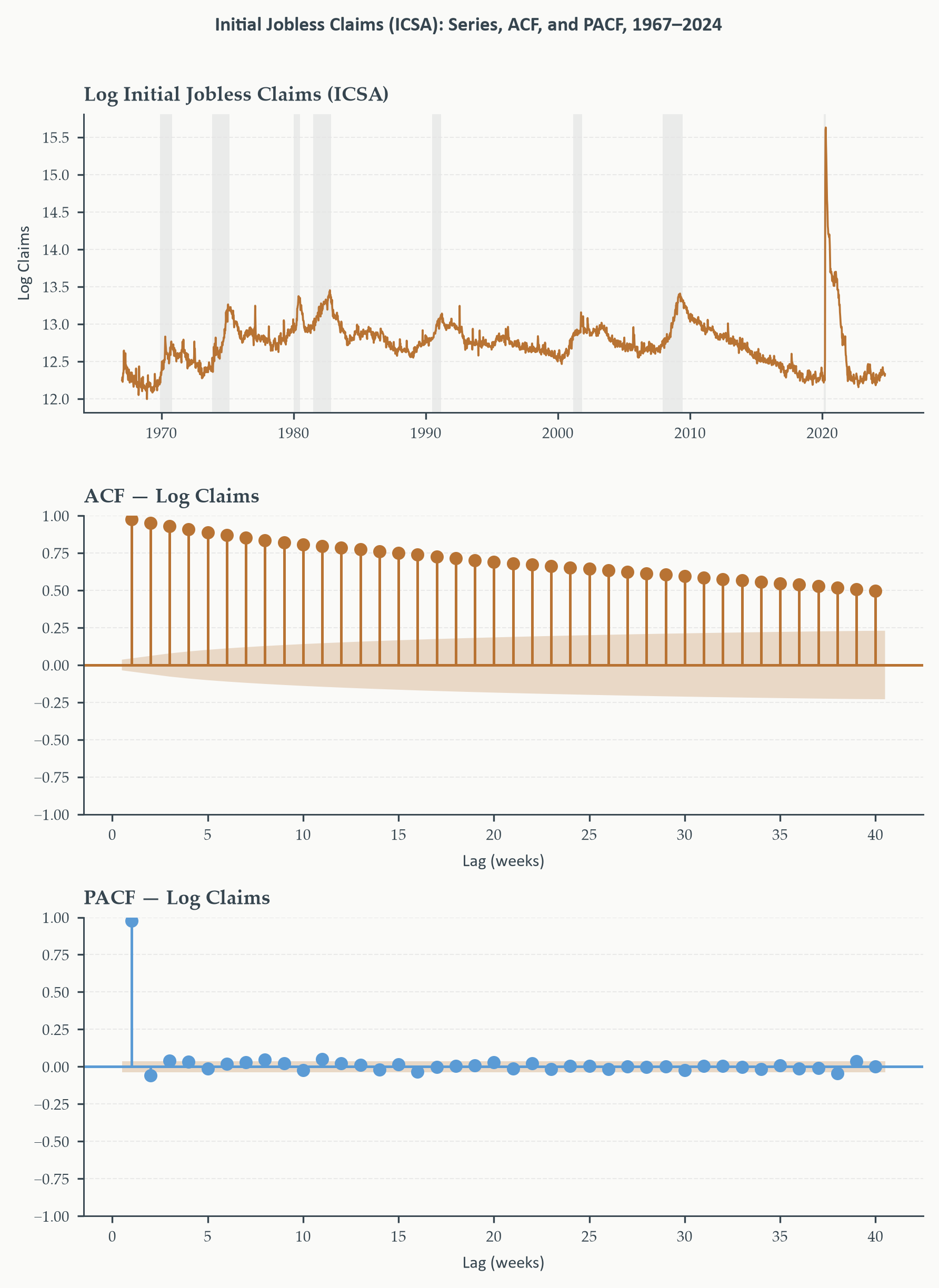
The ACF and PACF plot tells a clear story. The ACF decays slowly — remaining well
above zero for many lags — reflecting the high persistence of jobless claims.
When claims rise in a recession, they stay elevated; when they fall, the decline
is gradual. The PACF tells us how much of this persistence is directly
autoregressive: there is one dominant spike at lag 1, and everything beyond that
falls within or close to the confidence bands. This is almost exactly the pattern
predicted by an AR(1).
A word of caution before we fit anything. The full sample from 1967 to the present
spans nearly six decades of labour market history. The COVID-19 spike of 2020 is
visible to the naked eye. Less visible but equally important are the structural
changes of the late 1970s and early 1980s — the Volcker disinflation and the
deindustrialisation that permanently altered the composition of the workforce.
Whether a single AR model is the right representation for the full sample is a
genuine empirical question. We note the issue here and proceed with the full sample
to illustrate the identification and estimation workflow, but if we were writing a
research paper we would be more careful. Chapter 6 provides the tools — Chow tests,
Bai-Perron, Zivot-Andrews — for addressing this formally.
### The Yule-Walker Equations
For an AR($p$), there is a direct analytical link between the model's parameters
and its ACF. This link is useful for three reasons that we explain at the end of
this subsection; first, let us see where it comes from.
Subtract the mean and write the demeaned AR($p$) as:
$$\tilde{y}_t = \phi_1\tilde{y}_{t-1} + \cdots + \phi_p\tilde{y}_{t-p}
+ \varepsilon_t$$
Multiply both sides by $\tilde{y}_{t-h}$ and take expectations. The innovation
$\varepsilon_t$ is uncorrelated with any past value of the process, so
$\mathbb{E}[\varepsilon_t\tilde{y}_{t-h}] = 0$ for all $h \geq 1$. Dividing
through by $\gamma(0)$ gives the **[Yule-Walker equations](https://en.wikipedia.org/wiki/Autoregressive_model#Yule%E2%80%93Walker_equations)**:
$$\rho(h) = \phi_1\rho(h-1) + \phi_2\rho(h-2) + \cdots + \phi_p\rho(h-p),
\qquad h = 1, 2, \ldots, p \tag{3.7}$$
The structure is easiest to see in the first two cases.
**AR(1).** A single equation at $h=1$:
$$\rho(1) = \phi_1$$
The parameter equals the lag-1 autocorrelation directly — no algebra required.
This clean result is what makes the Yule-Walker system useful for intuition and
diagnostics: for an AR(1), $\hat\phi_1 \approx \hat\rho(1)$ and the first bar
of the PACF plot is almost a direct read-off of the AR coefficient.
**AR(2).** Two equations at $h = 1, 2$:
$$\begin{aligned}
\rho(1) &= \phi_1 + \phi_2\,\rho(1) \\
\rho(2) &= \phi_1\,\rho(1) + \phi_2
\end{aligned}$$
This $2 \times 2$ system has a unique solution whenever the process is stationary.
Solving the first equation for $\phi_1 = \rho(1)(1 - \phi_2)$ and substituting
into the second recovers both parameters from two observable autocorrelations.
**General AR($p$).** The system of $p$ equations can be written compactly as
$\mathbf{R}\boldsymbol\phi = \boldsymbol\rho$, where $\mathbf{R}$ is a $p\times p$
symmetric matrix whose $(i,j)$ entry is $\rho(|i-j|)$ and
$\boldsymbol\rho = (\rho(1),\ldots,\rho(p))'$. The solution
$\boldsymbol\phi = \mathbf{R}^{-1}\boldsymbol\rho$ exists and is unique when the
process is stationary.
Replacing population autocorrelations with sample estimates $\hat\rho(h)$ gives
the **Yule-Walker estimator** — closed-form, no iteration required. It is not
the most efficient estimator (MLE, Section 3.7, is preferred in practice), but
it matters for three reasons. First, it provides **starting values** for MLE
optimisation — a good first guess that prevents the numerical algorithm from
converging to a local optimum. Second, it is the foundation for computing the
**PACF**: the Durbin-Levinson algorithm generates PACF values by solving the
Yule-Walker system recursively for orders $p = 1, 2, 3, \ldots$, with the PACF
at lag $h$ being the last coefficient in the order-$h$ solution. Every PACF plot
in this chapter is, under the hood, a sequence of Yule-Walker solutions. Third,
it produces **clean theoretical results** — the AR(1) case above is the
canonical example, and results like it do not follow as easily from the
likelihood.
## The Wold Decomposition {#sec-wold}
Section 3.2 showed that any stationary AR($p$) can be written as an MA($\infty$):
an infinite weighted sum of current and past innovations. This is a useful result
for AR models — but it raises a deeper question. Is this just a quirk of the AR
family, or is there something more general going on? Could it be that *any*
covariance-stationary process — whatever its structure, however it was generated —
admits a representation as an infinite distributed lag of shocks?
The answer is yes, and it is one of the most important theoretical results in
time series analysis.
### The Theorem
::: {.callout-note}
## Theorem 3.1 — Wold Decomposition
Every covariance-stationary process $\{y_t\}$ with mean zero can be written as:
$$y_t = \underbrace{\sum_{j=0}^{\infty} \psi_j\,\varepsilon_{t-j}}_{\text{linearly indeterministic part}}
\;+\; \underbrace{\eta_t}_{\text{linearly deterministic part}} \tag{3.8}$$
where:
- $\psi_0 = 1$ and $\sum_{j=0}^{\infty}\psi_j^2 < \infty$ (the coefficients are
square-summable, ensuring the sum converges)
- $\{\varepsilon_t\} \sim WN(0, \sigma^2)$ are the **Wold innovations** — the
one-step-ahead forecast errors from the best linear predictor of $y_t$ given
its entire past
- $\eta_t$ is **linearly deterministic**: perfectly predictable from its own past
using a linear rule, and uncorrelated with $\varepsilon_s$ for all $s$ and $t$
:::
The decomposition separates $y_t$ into two orthogonal pieces: a stochastic part and a deterministic part. The deterministic part $\eta_t$ is perfectly predictable from the past, so it does not contribute to the process's unpredictability. The stochastic part, given by the infinite sum of innovations, captures all the unpredictable variation in $y_t$. The Wold innovations $\varepsilon_t$ are uncorrelated by construction, making them the fundamental building blocks of the process's randomness. For most economic time series, the deterministic part is either absent or trivially handled by demeaning, so we focus on the stochastic part. The key object is the MA($\infty$) representation: the sequence $\{\psi_j\}$ and the innovation process $\{\varepsilon_t\}$.
### Why This Matters
The [Wold theorem](https://en.wikipedia.org/wiki/Wold%27s_theorem) is not just a mathematical curiosity — it is the foundation on
which the entire ARMA family rests.
**It justifies MA models.** We have not yet introduced moving average models
formally, but the Wold theorem already tells us they are not arbitrary constructs.
An MA($q$) model is simply a Wold representation where all coefficients beyond lag
$q$ happen to be zero: $\psi_j = 0$ for $j > q$. The theorem says every stationary
process *has* a Wold representation; the MA($q$) says that representation *truncates*.
Whether that truncation is a good approximation to reality is an empirical question —
but the theoretical grounding is there.
**It justifies AR approximations.** Conversely, any truncated MA($\infty$) can be
approximated arbitrarily well by an AR($p$) of sufficiently high order. This is why
fitting an AR model to data that may not be truly autoregressive is not necessarily
wrong — under mild conditions, a high-order AR is a valid approximation to any
stationary process's Wold representation.
**It defines the innovation.** The Wold innovations $\varepsilon_t$ are a specific
object: the residuals from the best *linear* predictor of $y_t$ given all past
values. They are uncorrelated by construction, which is why they serve as the
building blocks. Importantly, they may not be independent — uncorrelated is weaker
than independent — but for forecasting purposes, uncorrelated innovations are
sufficient. The Wold theorem guarantees we can always find them.
**It connects to impulse responses.** The coefficients $\psi_j$ in the Wold
representation are the **impulse responses** of the process: $\psi_j$ is the effect
on $y_t$ of a unit shock to $\varepsilon_{t-j}$. In a stationary process, the
square-summability condition $\sum \psi_j^2 < \infty$ ensures impulse responses
eventually die out — shocks are transitory. This is the formal expression of what
it means for a process to have finite memory.
### What the Theorem Does Not Say
Two limitations are worth stating clearly.
First, the Wold representation is a linear representation. It says $y_t$ can be
written as a linear function of its innovations. It says nothing about nonlinear
structure: a process can have a Wold representation with serially uncorrelated
innovations and still contain nonlinear dependence — ARCH effects being the canonical
example. The squared innovations can be correlated even when the innovations
themselves are not. The Wold theorem is the foundation for the ARMA family; it is
not the foundation for GARCH models, which address a different question.
Second, the theorem is not constructive. It guarantees the representation exists but
does not tell us what $\psi_j$ are for a given process. We compute them either by
fitting a specific parametric model — AR, MA, ARMA — and reading off the implied
coefficients, or by estimating them directly from data using nonparametric methods.
Section 3.2 showed that any stationary AR has an MA($\infty$) representation. The
Wold theorem shows the converse is also true in a broad sense: any stationary
process has an MA($\infty$) representation. Together, these results tell us that
the MA family is not subordinate to the AR family — they are dual representations
of the same underlying structure. Section 3.4 develops MA models in their own
right, and Section 3.5 combines both into the ARMA family, where the duality
becomes a practical tool for building parsimonious models.
## Moving Average Models {#sec-ma}
Autoregressive models capture persistence through a direct feedback mechanism: the
past value of $y_t$ influences its future values. But there is a second, conceptually
distinct way that a series can exhibit temporal dependence — not through the level of
past observations, but through past *shocks*.
Think of a firm's inventory decisions. A supply disruption this month — an
$\varepsilon_t$ shock — forces the firm to draw down its stock. Next month, it
rebuilds. The *level* of output was not especially high last month, but the *shock*
last month directly influences this month's restocking behaviour. The series exhibits
memory not because output feeds back on itself, but because shocks propagate forward
through a specific mechanism for a limited number of periods, then stop. This is the
structure that moving average models are designed to capture.
### The MA(1) Model
The simplest moving average model is:
$$y_t = \mu + \varepsilon_t + \theta_1\varepsilon_{t-1}, \qquad
\varepsilon_t \sim WN(0,\sigma^2) \tag{3.9}$$
The current value of $y_t$ depends on the current innovation $\varepsilon_t$ and
the innovation from one period ago, $\varepsilon_{t-1}$. The parameter $\theta_1$
governs how strongly last period's shock feeds into today's value. Unlike the AR(1),
there is no feedback from past *levels* of $y_t$ — only from past *errors*.
The moments of the MA(1) are straightforward. The mean is $\mu$ by inspection.
For the variance:
$$\begin{aligned}
\sigma_y^2 &= \text{Var}(\varepsilon_t + \theta_1\varepsilon_{t-1}) \\
&= \text{Var}(\varepsilon_t) + \theta_1^2\,\text{Var}(\varepsilon_{t-1}) \\
&= \sigma^2 + \theta_1^2\sigma^2 \\
&= \sigma^2(1 + \theta_1^2)
\end{aligned}$$
where the second line uses the fact that $\varepsilon_t$ and $\varepsilon_{t-1}$
are uncorrelated. The autocovariance at lag 1:
$$\begin{aligned}
\gamma(1) &= \text{Cov}(y_t,\, y_{t-1}) \\
&= \text{Cov}(\varepsilon_t + \theta_1\varepsilon_{t-1},\;
\varepsilon_{t-1} + \theta_1\varepsilon_{t-2}) \\
&= \theta_1\,\text{Var}(\varepsilon_{t-1}) \\
&= \theta_1\sigma^2
\end{aligned}$$
The only nonzero cross-term is $\theta_1\,\text{Cov}(\varepsilon_{t-1},
\varepsilon_{t-1}) = \theta_1\sigma^2$; all other pairs of innovations are
uncorrelated. At lag 2 and beyond, $y_t$ and $y_{t-h}$ share no innovations in
common, so $\gamma(h) = 0$ for $h \geq 2$. The ACF of an MA(1) is therefore:
$$\rho(1) = \frac{\theta_1\sigma^2}{\sigma^2(1+\theta_1^2)}
= \frac{\theta_1}{1 + \theta_1^2}, \qquad \rho(h) = 0 \text{ for } h \geq 2
\tag{3.10}$$
This **finite, sharp cutoff** is the defining signature of MA models and the
mirror image of the AR's PACF cutoff. An MA(1) ACF drops to exactly zero after
lag 1 — not gradually, not approximately, but exactly. This makes MA models
immediately recognisable in ACF plots, and it is the key feature that distinguishes
them from AR models during identification.
::: {.callout-note}
## Definition 3.3 — The MA(1) Model
The **MA(1)** process is defined by:
$$y_t = \mu + \varepsilon_t + \theta_1\varepsilon_{t-1}, \qquad
\varepsilon_t \sim WN(0,\sigma^2)$$
It is always covariance-stationary regardless of the value of $\theta_1$, with:
$$\sigma_y^2 = \sigma^2(1+\theta_1^2), \qquad
\rho(1) = \frac{\theta_1}{1+\theta_1^2}, \qquad
\rho(h) = 0 \;\text{ for } h \geq 2$$
The ACF cuts off sharply after lag 1. The PACF tails off gradually.
:::
Three features of the MA(1) are worth pausing on.
First, notice that an MA model is *always* stationary — there is no stability
condition to check. Because $y_t$ is a finite linear combination of white noise
terms, it automatically inherits the stationarity of those terms. Stationarity is
free; it comes with the model structure. This is in sharp contrast to the AR
family, where stationarity requires a restriction on the parameters.
Second, stationarity and invertibility are logically independent conditions because
they govern different things. Stationarity is a property of the *output* of the
model — it asks whether $y_t$ has a stable, finite variance. For an MA model, this
is guaranteed by construction: $y_t$ is a finite sum of white noise terms, so its
variance is always finite regardless of $\theta_1$. Invertibility, by contrast, is
a property of the *innovation recovery* problem — it asks whether we can go
backwards from the observed data to reconstruct the innovations $\varepsilon_t$.
This is a condition on the MA polynomial $\theta(L)$ alone, and it can fail even
when the process is perfectly stationary. An MA(1) with $\theta_1 = 3$ is a
well-defined, stationary process with finite variance — it just happens to be one
whose innovations cannot be recovered from its observable history. The two
properties address different questions, which is why one can hold without the other.
Third, the formula for $\rho(1)$ reveals something subtle: $\rho(1)$ is bounded.
Taking the derivative of $\theta_1/(1+\theta_1^2)$ with respect to $\theta_1$ and
setting it to zero shows the maximum is $\pm 1/2$, achieved at $\theta_1 = \pm 1$.
An MA(1) can never produce a first-order autocorrelation larger than $1/2$ in
absolute value. This is a hard constraint with empirical implications: if you
observe $|\hat{\rho}(1)| > 0.5$ and the ACF cuts off after lag 1, the MA(1) is
not the right model.
### Invertibility
Stationarity is not the only condition we need to worry about for MA models.
There is a second requirement — **invertibility** — that has no counterpart in
the AR family.
To understand why, consider the MA(1) written in lag polynomial form:
$$y_t - \mu = \theta(L)\varepsilon_t, \qquad \theta(L) = 1 + \theta_1 L$$
Now ask: can we go the other direction and recover $\varepsilon_t$ from the
observed history of $y_t$? Formally, this requires inverting $\theta(L)$ to
write $\varepsilon_t = \theta(L)^{-1}(y_t - \mu)$. The inversion produces an
infinite series:
$$\varepsilon_t = (y_t - \mu) - \theta_1(y_{t-1} - \mu)
+ \theta_1^2(y_{t-2} - \mu) - \cdots$$
This series converges if and only if $|\theta_1| < 1$ — the characteristic root
of $\theta(L)$ must lie inside the unit circle, exactly as in the AR stationarity
condition. When this holds, the MA(1) is **invertible**: it can be rewritten as an
AR($\infty$) in $y_t$. When $|\theta_1| \geq 1$, the inversion diverges and the
MA(1) is non-invertible.
::: {.callout-note}
## Definition 3.4 — Invertibility
An MA($q$) model with lag polynomial $\theta(L) = 1 + \theta_1 L + \cdots +
\theta_q L^q$ is **invertible** if and only if all characteristic roots of
$\theta(L)$ lie strictly inside the unit circle — equivalently, the MA polynomial
can be inverted to yield a convergent AR($\infty$) representation.
For the MA(1): invertibility requires $|\theta_1| < 1$.
:::
Why does invertibility matter? Two reasons.
The first is **identification**. An MA(1) with parameter $\theta_1$ and an MA(1)
with parameter $1/\theta_1$ have exactly the same ACF — they are observationally
equivalent from the perspective of second moments alone. To see this, note that
$\rho(1) = \theta_1/(1+\theta_1^2)$ is unchanged when $\theta_1$ is replaced by
$1/\theta_1$. This means there are always two MA(1) models consistent with any
given ACF: one invertible ($|\theta_1| < 1$) and one non-invertible
($|\theta_1| > 1$). We conventionally pick the invertible one — not because it
fits better, but because it is the unique parameterisation that makes the
innovations recoverable from the observed data.
The second reason is **estimation and forecasting**. An invertible MA can be
approximated arbitrarily well by an AR of increasing order — a fact exploited
heavily in estimation and in computing forecasts. A non-invertible MA cannot. In
practice, statistical software enforces invertibility by default; it is worth
knowing why.
::: {.callout-note}
## Why Invertibility Matters — The Short Version
- **Identification:** without invertibility, two different parameter values
produce identical ACFs — the model is not uniquely recoverable from data.
- **Estimation:** innovations $\varepsilon_t$ are unobservable; invertibility
allows us to recover them from past $y_t$ values. A non-invertible MA process
*cannot* be estimated consistently from data.
- **Forecasting:** computing optimal forecasts requires the innovation sequence;
invertibility guarantees it is recoverable.
:::
### The MA(q) Model
The generalisation to $q$ lags is straightforward:
$$y_t = \mu + \varepsilon_t + \theta_1\varepsilon_{t-1} + \theta_2\varepsilon_{t-2}
+ \cdots + \theta_q\varepsilon_{t-q} = \mu + \theta(L)\varepsilon_t \tag{3.11}$$
where $\theta(L) = 1 + \theta_1 L + \cdots + \theta_q L^q$. The MA($q$) is always
stationary. It is invertible when all characteristic roots of $\theta(L)$ lie inside
the unit circle.
The ACF of an MA($q$) has the same defining property as the MA(1), now extended to
$q$ lags:
$$\rho(h) = \begin{cases}
\dfrac{\sum_{j=0}^{q-h}\theta_j\theta_{j+h}}{\sum_{j=0}^{q}\theta_j^2} &
h = 1, 2, \ldots, q \\[10pt]
0 & h > q
\end{cases} \tag{3.12}$$
where $\theta_0 = 1$ by convention. The ACF is nonzero for lags up to $q$ and
exactly zero for all lags beyond $q$. The PACF, by contrast, tails off gradually —
it never cuts off cleanly. This is the precise mirror image of the AR($p$).
To make the formula concrete, consider an MA(2) with $\theta_1 = 0.6$ and
$\theta_2 = 0.3$ — the same parameters used in the simulation of Section 3.4.
The denominator is $\theta_0^2 + \theta_1^2 + \theta_2^2 = 1 + 0.36 + 0.09 =
1.45$. At lag 1, the numerator sums the products of coefficients one step apart:
$\theta_0\theta_1 + \theta_1\theta_2 = (1)(0.6) + (0.6)(0.3) = 0.78$, giving
$\rho(1) = 0.78/1.45 = 0.538$. At lag 2, only the pair $(\theta_0, \theta_2)$
contributes: $\theta_0\theta_2 = (1)(0.3) = 0.30$, giving $\rho(2) = 0.30/1.45
= 0.207$. For all $h \geq 3$, $\rho(h) = 0$ exactly. This is exactly the pattern
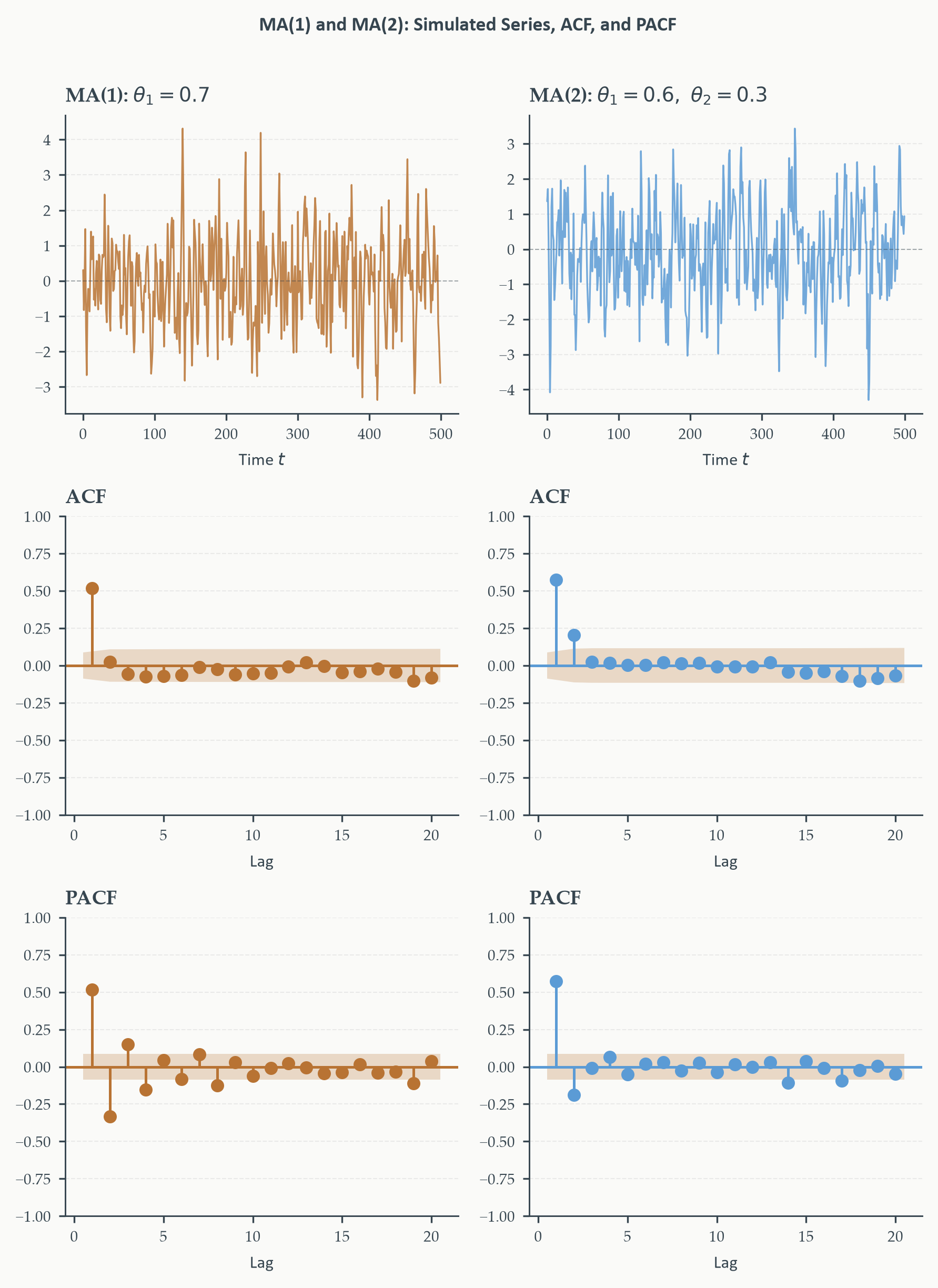
visible in the left-column ACF of the simulation figure: two significant bars
followed by near-zero values for all remaining lags.
| Model | ACF | PACF |
|:------|:----|:-----|
| AR($p$) | Tails off | Cuts off after lag $p$ |
| MA($q$) | Cuts off after lag $q$ | Tails off |
We expand this table in Section 3.6 to include ARMA models, where neither function
cuts off cleanly. For now, the key rule is: **a clean ACF cutoff points to MA;
a clean PACF cutoff points to AR**.
::: {.callout-note}
## Definition 3.5 — The MA($q$) Model
The **MA($q$)** process is:
$$y_t = \mu + \theta(L)\varepsilon_t, \qquad \theta(L) = 1 + \theta_1 L + \cdots
+ \theta_q L^q, \qquad \varepsilon_t \sim WN(0,\sigma^2)$$
Always stationary. Invertible when all characteristic roots of $\theta(L)$ lie
inside the unit circle. Its ACF cuts off sharply after lag $q$; its PACF tails
off gradually.
:::
### The MA(q) as an Infinite Autoregression
Just as the AR($p$) has an MA($\infty$) representation, an invertible MA($q$) has
an AR($\infty$) representation. Inverting $\theta(L)$ when all its roots are inside
the unit circle:
$$\varepsilon_t = \theta(L)^{-1}(y_t - \mu) = \pi(L)(y_t - \mu)$$
where $\pi(L) = 1 - \pi_1 L - \pi_2 L^2 - \cdots$ is an infinite lag polynomial
with coefficients that decay to zero. Rearranging:
$$y_t = \mu + \pi_1(y_{t-1}-\mu) + \pi_2(y_{t-2}-\mu) + \cdots + \varepsilon_t
\tag{3.13}$$
This representation reveals a fundamental difficulty in estimating MA models
directly: the right-hand side of the original MA equation (3.11) contains
$\varepsilon_{t-1}, \varepsilon_{t-2}, \ldots$ — past *innovations*, which are not
observed. We observe $y_t$, not $\varepsilon_t$. This makes the MA model
fundamentally different from a regression: we cannot simply form the design matrix
and run OLS, because the regressors do not exist in the data.
The AR($\infty$) representation in (3.13) is one way around this. Since the right-hand
side now contains only lagged *values* of $y_t$ — all of which are observed — we
can approximate (3.13) with a long but finite AR($K$), estimate it by OLS, and then
recover the MA parameters $\theta_1, \ldots, \theta_q$ from the estimated AR
coefficients. This works because the AR coefficients $\pi_1, \pi_2, \ldots$ are
deterministic functions of $\theta_1, \ldots, \theta_q$, so matching one set
identifies the other.
A more direct approach, and the one used in practice, is **iterative substitution**:
replace the unobservable innovations with estimated residuals, update the parameter
estimates, and repeat until convergence.
::: {.callout-note}
## How Do We Get $\hat\varepsilon_t$? Iterative Substitution
**Step 1.** Start with a large AR($K$) as a first guess. Extract the residuals
$e_t \approx \varepsilon_t$.
**Step 2.** Use $e_t$ as proxies for $\varepsilon_t$ in the MA equation. With the
current parameter estimates, construct fitted innovations recursively:
$$\hat\varepsilon_t = y_t - \hat\mu - \hat\theta_1\hat\varepsilon_{t-1} - \cdots
- \hat\theta_q\hat\varepsilon_{t-q}, \qquad \hat\varepsilon_0 = 0$$
**Step 3.** Update $\hat\theta_1, \ldots, \hat\theta_q$ by minimising the sum of
squared estimated residuals $\sum_t \hat\varepsilon_t^2$.
**Step 4.** Repeat Steps 2–3 until the parameters stop changing.
**Result.** *Estimated residuals stand in for true innovations*, improving with each
iteration. MLE (Section 3.7) performs this rigorously with a distributional
assumption, handling initialisation properly — but the intuition is identical.
:::
Invertibility is what guarantees this iteration converges. If the MA polynomial is
not invertible, the estimated innovations do not stabilise and the procedure breaks
down — the deepest reason invertibility matters for estimation, not just identification.
### Python: The MA Signature in Simulated Data
The ACF cutoff for MA models is clean enough in theory. It is worth seeing it in
simulated data before we use it as a diagnostic tool on real series, to calibrate
how sharp the cutoff looks in finite samples and how confidently we can read it off
an ACF plot.
```{python}
#| label: fig-ma-acf
#| fig-cap: "Simulated MA(1) and MA(2) processes ($T = 500$) and their sample
#| ACFs and PACFs. Left column: MA(1) with $\\theta_1 = 0.7$. Right column:
#| MA(2) with $\\theta_1 = 0.6$, $\\theta_2 = 0.3$. Top row: time series.
#| Middle row: sample ACF — the cutoff after lag 1 (left) and lag 2 (right)
#| is visible, though sampling noise means a few small spikes appear beyond
#| the cutoff. Bottom row: sample PACF — tailing off gradually, with no clean
#| cutoff. The contrast with the AR PACF pattern from Section 3.2 is stark."
#| fig-width: 6
#| fig-height: 8
#| code-fold: true
#| code-summary: "Show code — MA ACF/PACF"
from statsmodels.tsa.arima_process import ArmaProcess

rng = np.random.default_rng(seed=42)
T   = 500

# MA(1): theta_1 = 0.7  →  arparams = [1], maparams = [1, 0.7]
ma1_process = ArmaProcess(ar=np.array([1]),
                          ma=np.array([1, 0.7]))
ma1_sim     = ma1_process.generate_sample(nsample=T, distrvs=rng.standard_normal)

# MA(2): theta_1 = 0.6, theta_2 = 0.3
ma2_process = ArmaProcess(ar=np.array([1]),
                          ma=np.array([1, 0.6, 0.3]))
ma2_sim     = ma2_process.generate_sample(nsample=T, distrvs=rng.standard_normal)

fig, axes = plt.subplots(3, 2, figsize=(6, 8))

labels   = [r"MA(1): $\theta_1 = 0.7$",
            r"MA(2): $\theta_1 = 0.6,\ \theta_2 = 0.3$"]
sims     = [ma1_sim, ma2_sim]
colors   = [EO_COPPER, EO_SKYBLUE]

for col, (sim, label, color) in enumerate(zip(sims, labels, colors)):

    # Time series
    ax = axes[0, col]
    ax.plot(sim, color=color, lw=0.8, alpha=0.85)
    ax.axhline(0, color=EO_CHARCOAL, lw=0.5, ls="--", alpha=0.4)
    ax.set_title(label)
    ax.set_xlabel("Time $t$")
    eo_style_ax(ax)

    # ACF
    ax = axes[1, col]
    plot_acf(sim, lags=20, ax=ax,
             color=color, vlines_kwargs={"colors": color},
             title="ACF", zero=False, alpha=0.05)
    ax.set_xlabel("Lag")
    eo_style_ax(ax)
    for line in ax.lines:
        if line.get_linestyle() == "--":
            line.set_color(EO_TERRACOTTA)
            line.set_linewidth(0.8)

    # PACF
    ax = axes[2, col]
    plot_pacf(sim, lags=20, ax=ax,
              color=color, vlines_kwargs={"colors": color},
              title="PACF", zero=False, alpha=0.05)
    ax.set_xlabel("Lag")
    eo_style_ax(ax)
    for line in ax.lines:
        if line.get_linestyle() == "--":
            line.set_color(EO_TERRACOTTA)
            line.set_linewidth(0.8)

eo_suptitle(fig, "MA(1) and MA(2): Simulated Series, ACF, and PACF")
fig.tight_layout()
plt.show()
```
The simulation confirms the theory, with one caveat worth noting: even with $T=500$
observations, the ACF does not drop to *exactly* zero beyond the cutoff lag. A few
bars exceed the confidence bands by chance, and many more fall just inside them
with nonzero point estimates. In finite samples, the signal we are looking for is
not a perfect flat line at zero but a sharp drop followed by a pattern
indistinguishable from sampling noise. Learning to read this — to distinguish a
genuine cutoff from sampling fluctuation — is part of the identification skill
developed in Section 3.6.
The PACF panels show the complementary pattern: no clean cutoff anywhere, just a
gradual decay with occasional spikes that reflect the complex infinite AR
representation underlying every MA model. An ACF that drops after lag 2 with a PACF that shows no obvious cutoff is the
signature of an MA(2).
## ARMA Models {#sec-arma}
### Combining AR and MA: The Case for a Mixed Model
Sections 3.2 and 3.4 introduced two complementary model families. AR models capture
persistence through feedback from past levels. MA models capture shock propagation
through a finite distributed lag of innovations. Both are useful, but each has a
limitation when used alone.
A pure AR($p$) can represent any stationary process via a sufficiently long lag
— this is the Wold theorem — but it may require many lags to do so adequately. A
process whose true structure is MA(1) needs, in principle, an AR($\infty$) to
represent it exactly. Approximating that with an AR(10) or AR(20) is wasteful:
nineteen or more parameters to represent what is fundamentally a one-parameter
structure. Conversely, a pure MA($q$) can become unwieldy for processes with rich
autoregressive structure.
The **[ARMA($p$,$q$)](https://en.wikipedia.org/wiki/Autoregressive_moving-average_model)** model combines both components:
$$\phi(L)\,y_t = \mu^* + \theta(L)\varepsilon_t \tag{3.14}$$
where $\phi(L) = 1 - \phi_1 L - \cdots - \phi_p L^p$ is the AR polynomial and
$\theta(L) = 1 + \theta_1 L + \cdots + \theta_q L^q$ is the MA polynomial.
The constant $\mu^*$ deserves a brief explanation. If $\mu = \mathbb{E}[y_t]$ is
the unconditional mean, applying $\phi(L)$ to both sides of $y_t = \mu +
\tilde{y}_t$ (where $\tilde{y}_t = y_t - \mu$ is the demeaned process) gives
$\phi(L)y_t = \phi(L)\mu + \phi(L)\tilde{y}_t$. Since $\phi(L)\mu =
(1 - \phi_1 - \cdots - \phi_p)\mu = \phi(1)\mu$, the intercept that appears on
the right-hand side of the ARMA equation is not $\mu$ itself but
$$\mu^* = \phi(1)\,\mu = (1 - \phi_1 - \cdots - \phi_p)\,\mu$$
This matters in practice: when you fit an ARMA model, the reported
intercept is $\hat\mu^*$, not $\hat\mu$. To recover the estimated unconditional
mean, divide by $\hat\phi(1) = 1 - \hat\phi_1 - \cdots - \hat\phi_p$. For a
pure MA model, $\phi(L) = 1$ so $\phi(1) = 1$ and $\mu^* = \mu$ — the intercept
is the mean directly. Written out explicitly:
$$y_t = \mu^* + \phi_1 y_{t-1} + \cdots + \phi_p y_{t-p}
+ \varepsilon_t + \theta_1\varepsilon_{t-1} + \cdots + \theta_q\varepsilon_{t-q}
\tag{3.15}$$
The process is covariance-stationary when all characteristic roots of $\phi(L)$
lie inside the unit circle, and invertible when all characteristic roots of
$\theta(L)$ lie inside the unit circle. The stationarity condition depends only on
the AR part; the invertibility condition depends only on the MA part. The two
conditions are independent of each other, just as we saw for stationarity and
invertibility in Section 3.4.
::: {.callout-note}
## Definition 3.6 — The ARMA($p$,$q$) Model
The **ARMA($p$,$q$)** process is:
$$\phi(L)\,y_t = \mu^* + \theta(L)\varepsilon_t, \qquad
\varepsilon_t \sim WN(0,\sigma^2)$$
where $\phi(L) = 1 - \phi_1 L - \cdots - \phi_p L^p$ and
$\theta(L) = 1 + \theta_1 L + \cdots + \theta_q L^q$.
**Stationary** when all characteristic roots of $\phi(L)$ lie inside the unit
circle. **Invertible** when all characteristic roots of $\theta(L)$ lie inside
the unit circle. The ACF and PACF both tail off gradually — neither cuts off
sharply.
:::
### Parsimony: Why ARMA Models Earn Their Parameters
The motivation for combining AR and MA components is parsimony — achieving an
adequate representation of the data's dynamic structure with the fewest parameters.
The classic illustration is the **ARMA(1,1)**:
$$y_t = \mu^* + \phi_1 y_{t-1} + \varepsilon_t + \theta_1\varepsilon_{t-1}
\tag{3.16}$$
This two-parameter model (plus $\mu^*$ and $\sigma^2$) can approximate processes
that would require a much longer pure AR or pure MA. The AR component handles
the persistent, slowly decaying part of the autocorrelation structure; the MA
component handles the shape of the initial decay. Together, they provide a flexible
template that is often sufficient for economic time series with moderate complexity.
A useful heuristic: if the ACF and PACF both tail off gradually from the first lag —
neither showing a clean cutoff — an ARMA model is likely more parsimonious than
either an AR or MA alone. The precise orders $p$ and $q$ are then chosen by the
information criteria discussed in Section 3.6.
### The Cancellation Problem
The efficiency of the ARMA representation comes with one important caveat. If the AR
polynomial $\phi(L)$ and the MA polynomial $\theta(L)$ share a common characteristic
root, that root cancels from both sides of equation (3.14):
$$\frac{\theta(L)}{\phi(L)} = \frac{\theta(L) / (1 - \lambda L)}{\phi(L) / (1 - \lambda L)}$$
The result is a lower-order ARMA with identical statistical properties. Writing
the unreduced form wastes parameters, inflates standard errors, and can cause
numerical instability in estimation — the likelihood surface becomes flat along
the direction of the common root, making optimisation unreliable.
::: {.callout-warning icon=false}
## The Cancellation Problem
An ARMA($p$,$q$) specification is **parameter redundant** if $\phi(L)$ and
$\theta(L)$ share a common characteristic root. The true model is then a lower-order
ARMA($p-k$,$q-k$) for some $k \geq 1$. Symptoms in practice: near-cancelling root
pairs in the estimated polynomials, large standard errors on some coefficients, and
poor numerical convergence. The remedy is to reduce the order of both polynomials
until no common roots remain.
:::
In practice, parameter redundancy is rare when models are selected carefully by
information criteria — the penalty for extra parameters discourages overfitting.
But it is worth knowing the pathology exists, because fitting an ARMA(2,1) to a
series whose true model is AR(1) is a common beginner mistake when ACF/PACF
patterns are misread.
### ACF and PACF of an ARMA: Neither Cuts Off
The identification picture for ARMA models is more complex than for pure AR or MA.
Because both polynomials contribute to the autocovariance structure, neither the
ACF nor the PACF cuts off sharply. Both tail off, typically as a mixture of
exponentials and damped sinusoids determined by the roots of $\phi(L)$.
This makes ARMA models harder to identify from ACF/PACF plots alone than pure AR
or MA models. The identification table now reads:
| Model | ACF | PACF |
|:------|:----|:-----|
| AR($p$) | Tails off | Cuts off after lag $p$ |
| MA($q$) | Cuts off after lag $q$ | Tails off |
| ARMA($p$,$q$) | Tails off after lag $q-p$ | Tails off after lag $p-q$ |
| White noise | Zero at all lags | Zero at all lags |
The ARMA row deserves comment. After lag $\max(p,q)$, the ACF follows a pattern
governed entirely by the AR roots — it decays as a mixture of $\phi_1^h, \phi_2^h,
\ldots$ The MA component affects the shape of the ACF at early lags but leaves no
trace beyond lag $q$. Similarly for the PACF. In practice, "tails off from the
start" for both functions is the working rule for identifying ARMA candidates, and
information criteria then determine the order.
### Python: AR, MA, and ARMA — ACF Patterns Side by Side
The clearest way to internalise the identification table is to see all three model
families plotted together. The figure below simulates an AR(1), an MA(1), and an
ARMA(1,1) with comparable persistence, and plots their ACFs and PACFs side by side.
```{python}
#| label: fig-arma-comparison
#| fig-cap: "ACF and PACF for simulated AR(1), MA(1), and ARMA(1,1) processes
#| ($T = 500$). AR(1) with $\\phi_1 = 0.7$: PACF cuts off sharply after lag 1,
#| ACF tails off. MA(1) with $\\theta_1 = 0.7$: ACF cuts off after lag 1,
#| PACF tails off. ARMA(1,1) with $\\phi_1 = 0.6$, $\\theta_1 = 0.4$: both
#| ACF and PACF tail off from the start — neither shows a clean cutoff.
#| The identification table comes to life: each model class has a distinct
#| signature."
#| fig-width: 6
#| fig-height: 7
#| code-fold: true
#| code-summary: "Show code — AR/MA/ARMA comparison"
from statsmodels.tsa.arima_process import ArmaProcess

rng = np.random.default_rng(seed=99)
T   = 500

# AR(1): phi_1 = 0.7
ar1 = ArmaProcess(ar=np.array([1, -0.7]), ma=np.array([1]))
ar1_sim = ar1.generate_sample(nsample=T, distrvs=rng.standard_normal)

# MA(1): theta_1 = 0.7
ma1 = ArmaProcess(ar=np.array([1]), ma=np.array([1, 0.7]))
ma1_sim = ma1.generate_sample(nsample=T, distrvs=rng.standard_normal)

# ARMA(1,1): phi_1 = 0.6, theta_1 = 0.4
arma11 = ArmaProcess(ar=np.array([1, -0.6]), ma=np.array([1, 0.4]))
arma11_sim = arma11.generate_sample(nsample=T, distrvs=rng.standard_normal)

specs  = [
    (ar1_sim,    r"AR(1): $\phi_1=0.7$",                      EO_COPPER),
    (ma1_sim,    r"MA(1): $\theta_1=0.7$",                    EO_SKYBLUE),
    (arma11_sim, r"ARMA(1,1): $\phi_1=0.6,\ \theta_1=0.4$",  EO_SAGE),
]

fig, axes = plt.subplots(2, 3, figsize=(6, 7), sharey="row")

for col, (sim, label, color) in enumerate(specs):

    # ACF
    ax = axes[0, col]
    plot_acf(sim, lags=20, ax=ax,
             color=color, vlines_kwargs={"colors": color},
             title=label, zero=False, alpha=0.05)
    ax.set_xlabel("Lag")
    if col == 0:
        ax.set_ylabel("ACF")
    eo_style_ax(ax)
    for line in ax.lines:
        if line.get_linestyle() == "--":
            line.set_color(EO_TERRACOTTA)
            line.set_linewidth(0.8)

    # PACF
    ax = axes[1, col]
    plot_pacf(sim, lags=20, ax=ax,
              color=color, vlines_kwargs={"colors": color},
              title="", zero=False, alpha=0.05)
    ax.set_xlabel("Lag")
    if col == 0:
        ax.set_ylabel("PACF")
    eo_style_ax(ax)
    for line in ax.lines:
        if line.get_linestyle() == "--":
            line.set_color(EO_TERRACOTTA)
            line.set_linewidth(0.8)

eo_suptitle(fig, "ACF and PACF: AR(1), MA(1), ARMA(1,1) — $T=500$")
fig.tight_layout()
plt.show()
```
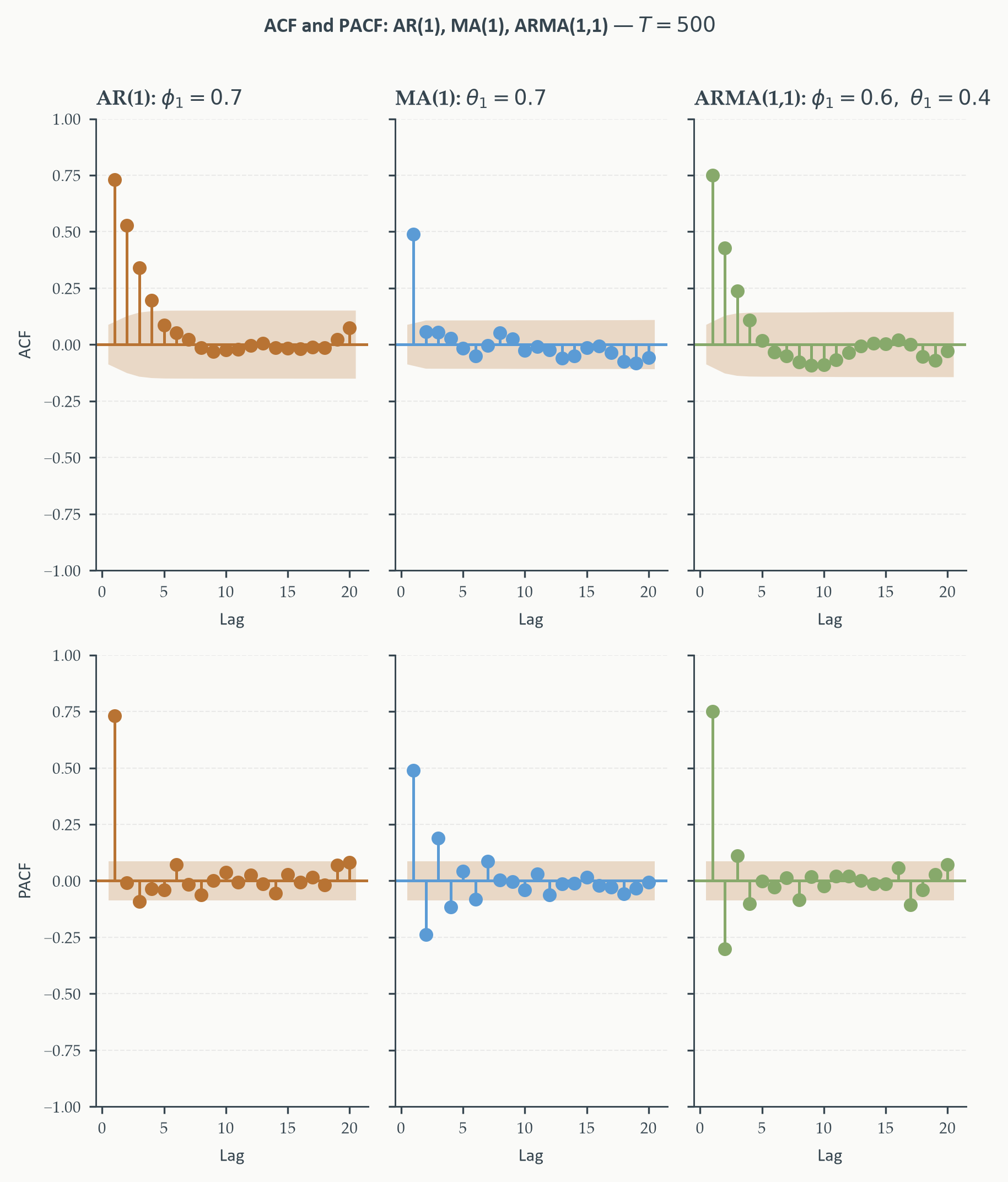
The figure makes the identification table tangible. The AR column shows the PACF
spike at lag 1 followed by near-zero values — the clean cutoff is unmistakable.
The MA column shows the ACF spike at lag 1 and a PACF that decays without
truncating. The ARMA column shows both functions declining from the first lag, with
no cutoff in either direction. These three patterns are what practitioners learn to
recognise before reaching for an information criterion.
## Model Identification {#sec-identification}
### The Identification Problem
We now have three model families — AR, MA, ARMA — and a set of theoretical
predictions about what their ACF and PACF patterns look like. The **identification
problem** is the reverse question: given a sample ACF and PACF computed from real
data, which model class does the pattern suggest, and what order?
This is not a mechanical exercise. Real data are finite, noisy, and generated by
processes far more complex than any parametric model. The ACF and PACF provide
evidence, not verdicts. The skill we develop in this section is reading that
evidence systematically — combining the pattern-recognition rules from Sections
3.2–3.5 with formal model selection criteria and the discipline of the [Box-Jenkins
workflow](https://en.wikipedia.org/wiki/Box%E2%80%93Jenkins_method).
### Step 1: Stationarity
Before any model can be identified, the series must be stationary. This step was
covered in Chapter 1 (ADF and KPSS tests) and is a precondition for everything that
follows. In practice:
- Plot the series. A visible trend or expanding variance is an immediate signal.
- Examine the ACF. A very slowly decaying ACF — remaining large at lags 10, 20,
or more — is the visual fingerprint of a unit root or near-unit-root process.
- Confirm with ADF and KPSS. Use them jointly: ADF failure to reject combined with
KPSS rejection is the strongest evidence for a unit root.
If the series is nonstationary, difference it. Log-differencing is appropriate for
series with exponential growth (GDP, prices, asset prices). First differencing
suffices for most economic series. Because nonstationarity is so consequential
for every subsequent modelling step — and because unit root testing has its own
subtleties of test specification, critical values, and power — we devote detailed
attention to it in Chapter 4, where the ARIMA framework makes the treatment
of integrated series fully explicit.
### Step 2: ACF and PACF Pattern Recognition
With a stationary series in hand, compute the sample ACF and PACF and apply the
identification table from Section 3.5:
| Pattern | Suggested model |
|:--------|:----------------|
| PACF cuts off after lag $p$; ACF tails off | AR($p$) |
| ACF cuts off after lag $q$; PACF tails off | MA($q$) |
| Both ACF and PACF tail off | ARMA($p$,$q$) — use IC to choose orders |
| Neither shows significant structure | White noise — no model needed |
Reading ACF and PACF plots requires calibrated judgment. A few practical rules help.
**Confidence bands are guides, not gates.** The standard 95% bands are
$\pm 1.96/\sqrt{T}$. A bar that barely crosses the band may be noise; a cluster of
bars all exceeding the band at the same lags is signal. Look at the pattern, not
individual bars.
**Seasonal spikes are not AR or MA structure.** Regular spikes at lags 4, 8, 12
(quarterly) or 12, 24, 36 (monthly) indicate seasonal dependence. This requires a
seasonal model (SARIMA, Chapter 4), not a higher-order ARMA.
**Start small.** Begin with the simplest model consistent with the pattern. An AR(1)
or ARMA(1,1) often fits as well as higher-order alternatives once information
criteria penalise for complexity. Overfitting is a real risk.
### Step 3: The Box-Jenkins Workflow
The ACF/PACF pattern gives a tentative identification. The Box-Jenkins workflow
structures what comes next:
::: {.callout-note}
## The Box-Jenkins Workflow
1. **Identification** — Inspect the ACF and PACF of the stationary series.
Tentatively select model class (AR, MA, ARMA) and one or more candidate orders.
2. **Estimation** — Fit the candidate model(s) by maximum likelihood (Section 3.7).
3. **Diagnostics** — Check that residuals behave like white noise (Section 3.8).
If significant ACF/PACF structure remains in the residuals, the model has not
captured all predictable structure — return to step 1.
4. **Selection** — Among models that pass diagnostics, choose by information
criteria (below). Prefer the most parsimonious adequate model.
5. **Forecasting** — Use the selected model to produce point forecasts and
prediction intervals (Section 3.9).
:::
The workflow is iterative. Diagnostics frequently send us back to identification
with new information: residual ACF spikes at lag $q$ suggest a missing MA term;
residual PACF spikes at lag $p$ suggest a missing AR term. This back-and-forth is
normal — it is how practitioners refine models rather than a sign that something
has gone wrong.
### Step 4: Information Criteria
When multiple models pass diagnostics, we need a principled way to choose among
them. The problem is that adding parameters always improves in-sample fit —
a model with more lags will always explain more of the variation in the estimation
sample. What we want is a model that generalises well to new data, and that requires
penalising complexity.
[Information criteria](https://en.wikipedia.org/wiki/Model_selection#Criteria) (IC) formalise this tradeoff. They all take the same conceptual
form:
$$\text{IC} = -2\,\hat\ell + \text{penalty}(k, T)$$
where $\hat\ell$ is the maximised log-likelihood of the fitted model, $k$ is the
number of estimated parameters, and $T$ is the sample size. The first term rewards
fit; the second penalises complexity. A lower value of IC is better. The three
criteria in common use differ only in how steeply they penalise:
::: {.callout-note}
## Information Criteria for ARMA Model Selection
| Criterion | Formula | Penalty per parameter |
|:----------|:--------|:----------------------|
| AIC (Akaike) | $-2\hat\ell + 2k$ | $2$ |
| BIC (Bayesian / Schwarz) | $-2\hat\ell + k\ln T$ | $\ln T$ |
| HQ (Hannan-Quinn) | $-2\hat\ell + 2k\ln\ln T$ | $2\ln\ln T$ |
$k$ = number of estimated parameters (AR lags + MA lags + intercept + variance);
$T$ = sample size. Select the model with the **lowest** value.
:::
The conceptual story behind each criterion is the same: start with the
log-likelihood as the measure of fit, then charge a fee for each additional
parameter. AIC charges a flat fee of 2 per parameter regardless of sample size —
it is relatively forgiving of complexity and tends to select larger models. BIC
charges $\ln T$ per parameter, which grows with sample size — at $T = 100$ the
penalty is about 4.6 per parameter, already more than twice AIC's. BIC therefore
favours more parsimonious models as the sample grows, and is **consistent**: in
large samples it selects the true model order with probability approaching 1, if
the true model is in the candidate set. HQ sits between them, with a penalty that
grows with sample size but more slowly than BIC.
The practical implications:
- If the goal is **forecasting**, AIC often performs better in finite samples
because it tolerates slightly larger models that capture more nuance.
- If the goal is **inference about model order** — how many lags does this
process truly have? — BIC's consistency property makes it the preferred criterion.
- HQ is a reasonable compromise, less commonly used in economics than AIC or BIC
but theoretically well-motivated.
None of the three criteria is uniformly best. Practitioners often compute all three
and pay attention when they agree. When they disagree, the disagreement itself is
informative — it usually means the data do not strongly discriminate between model
orders, and a simpler model is defensible.
**Why not adjusted $R^2$?** The natural question is whether the adjusted $R^2$ — which does penalise for extra parameters — can serve
as a model selection criterion here. It is a reasonable instinct: adjusted $R^2$
imposes a penalty of one degree of freedom per added regressor, so it does not
mechanically prefer the most heavily parameterised model. The problem is that the
penalty is ad hoc. Adjusted $R^2$ penalises each parameter by the same fixed
amount regardless of sample size, regardless of the model's intended use, and
without any connection to the statistical properties we actually care about —
such as consistency in recovering the true order, or minimising forecast mean
squared error. Information criteria derive their penalty terms from likelihood
theory and, in the case of BIC and HQ, from large-sample optimality results.
They also apply naturally to MA and ARMA models, where the concept of $R^2$ is
less natural because the innovations are not directly observed. In time series
econometrics, information criteria are the standard tool; adjusted $R^2$ belongs
in the cross-sectional regression toolkit.
### Python: Applying the Workflow to Initial Jobless Claims
We return to the ICSA series from Section 3.2. The ACF and PACF already suggested
AR(1) dynamics. We now apply the full Box-Jenkins workflow: fit several candidate
models, compute information criteria, and select.
Before fitting, we address the structural break issue flagged in Section 3.2.
The COVID-19 spike of 2020 is a severe outlier that will distort any model estimated
on the full sample. For the purposes of this identification exercise, we restrict
the sample to the pre-pandemic period, 1967–2019. This is a pragmatic choice, not
a permanent one — Chapter 4 provides formal tools for testing and handling breaks.
```{python}
#| label: tbl-icsa-ic
#| code-fold: true
#| code-summary: "Show code — ARMA model selection"
# Restrict to pre-pandemic sample
icsa_pre = icsa.loc[:"2019-12-31", "Log Claims"].dropna()

results = []
for p in range(0, 4):
    for q in range(0, 4):
        if p == 0 and q == 0:
            continue
        try:
            mod = ARIMA(icsa_pre, order=(p, 0, q)).fit()
            results.append({
                "Model":  f"ARMA({p},{q})",
                "Params": p + q + 2,        # AR + MA + intercept + sigma^2
                "AIC":    round(mod.aic, 1),
                "BIC":    round(mod.bic, 1),
                "HQ":     round(mod.hqic, 1),
            })
        except Exception:
            pass

ic_df = pd.DataFrame(results).sort_values("AIC").reset_index(drop=True)

# Mark best (minimum) in each IC column
def fmt_col(col):
    mn = col.min()
    return col.apply(lambda x: f"**{x}**" if x == mn else str(x))

ic_display = ic_df.copy()
for c in ["AIC", "BIC", "HQ"]:
    ic_display[c] = fmt_col(ic_df[c])

print(ic_display.to_string(index=False))
```
*Information criteria for ARMA($p$,$q$) models fitted to log initial jobless
claims (ICSA), 1967–2019. Sorted by AIC. Bold entries mark the minimum in each
column.*
The table illustrates a common feature of real-data identification: the three
criteria do not agree. AIC selects ARMA(3,3) — the largest model in the grid
— while BIC and HQ both select ARMA(1,2). This disagreement is itself informative.
The AIC result reflects its relatively forgiving penalty: with nearly 2,800 weekly
observations, the gain in log-likelihood from adding higher-order AR and MA terms
is large enough in absolute terms to justify the cost under AIC's flat
$2k$ penalty. The BIC and HQ results reflect a steeper penalty that grows with
sample size — $\ln T \approx 7.9$ per parameter here — and finds that the
marginal improvement in fit from ARMA(3,3) over ARMA(1,2) does not clear that
bar.
Which should we trust? For a forecasting application, AIC's preference for
ARMA(3,3) is defensible — it may capture richer short-run dynamics that improve
near-term predictions. For inference about the true order of the process, BIC's
consistency property gives it the edge, and ARMA(1,2) is the more credible
structural characterisation. The disagreement also signals that the data do not
sharply discriminate between these specifications: the likelihood differences are
modest, and a practitioner could defend either choice.
Notice that the ARMA(1,2) preferred by BIC and HQ is richer than the AR(1) the
ACF/PACF suggested. This is a reminder that visual identification is a first pass,
not a final answer. The PACF spike at lag 1 identified the dominant AR component
correctly; the MA(2) term captures residual structure that the pure AR(1) misses.
Section 3.7 fits the ARMA(1,2) by maximum likelihood and interprets the output.
## Estimation {#sec-estimation}
### The Problem of Estimation
Identification gives us a candidate model — an ARMA($p$,$q$) with specific orders.
Estimation is the step that turns that candidate into a fitted model: it finds
the parameter values $(\phi_1,\ldots,\phi_p,\,\theta_1,\ldots,\theta_q,\,\mu,\,
\sigma^2)$ that are most consistent with the observed data. There are two main
approaches — conditional least squares and maximum likelihood — that give identical
answers asymptotically but differ in small samples. In practice, maximum likelihood
is the standard, and it is what `statsmodels` uses by default.
### Conditional Least Squares
The simplest approach is **conditional least squares (CLS)**. For an ARMA($p$,$q$),
start from the model written as:
$$\varepsilon_t = y_t - \mu^* - \phi_1 y_{t-1} - \cdots - \phi_p y_{t-p}
- \theta_1\varepsilon_{t-1} - \cdots - \theta_q\varepsilon_{t-q}$$
CLS minimises the sum of squared residuals $\sum_{t} \hat\varepsilon_t^2$, treating
the pre-sample innovations as zero: $\hat\varepsilon_0 = \hat\varepsilon_{-1} =
\cdots = 0$. This conditioning on the presample is where the name comes from, and
it is the source of the small-sample inaccuracy: setting unobserved initial
innovations to zero introduces a bias that shrinks as $T$ grows. For most economic
applications with samples of several hundred observations or more, the bias is
negligible. For short samples or models with large MA coefficients, MLE is clearly
preferable.
CLS is implemented iteratively using the same logic as Section 3.4: at each
iteration, estimated residuals $\hat\varepsilon_{t-j}$ stand in for the
unobserved true innovations, the parameters are updated, and the cycle repeats
until convergence. It is fast, transparent, and useful for understanding what
estimation is doing — but it is not the modern standard.
### Maximum Likelihood Estimation
The intuition behind **maximum likelihood estimation (MLE)** is best approached
from a question: given a dataset, which parameter values would have made this
particular sequence of observations most probable? Think of flipping a coin ten
times and observing eight heads. A fair coin ($p=0.5$) could produce this, but it
is not the most likely explanation — a coin with $p=0.8$ would make eight heads
much more probable. MLE finds the parameter values that assign the highest
probability to the data we actually observed. It is, in this sense, the most
natural way to let the data speak.
For an ARMA($p$,$q$) with Gaussian innovations $\varepsilon_t \sim N(0,\sigma^2)$,
the probability of observing a particular innovation $\varepsilon_t$ is the
Gaussian density $f(\varepsilon_t) \propto \exp(-\varepsilon_t^2 / 2\sigma^2)$.
Since innovations are uncorrelated, the joint probability of observing the entire
sequence $\varepsilon_1, \ldots, \varepsilon_T$ is the product of individual
densities. Taking logarithms — which turns products into sums and makes
optimisation tractable — the **log-likelihood** is:
$$\ell(\phi,\theta,\mu,\sigma^2) = -\frac{T}{2}\ln(2\pi)
- \frac{T}{2}\ln\sigma^2
- \frac{1}{2\sigma^2}\sum_{t=1}^{T}\varepsilon_t(\phi,\theta,\mu)^2 \tag{3.17}$$
where the innovations are not free parameters but are **computed from the data
and the model parameters** recursively:
$$\varepsilon_t(\phi,\theta,\mu) = y_t - \mu^*
- \phi_1 y_{t-1} - \cdots - \phi_p y_{t-p}
- \theta_1\hat\varepsilon_{t-1} - \cdots - \theta_q\hat\varepsilon_{t-q}
\tag{3.18}$$
with $\mu^* = (1 - \phi_1 - \cdots - \phi_p)\mu$ as established in Section 3.5.
The mean $\mu$ enters through $\mu^*$: a different value of $\mu$ shifts every
innovation, changing the sum of squares in (3.17) and therefore the likelihood.
MLE jointly chooses $(\phi, \theta, \mu, \sigma^2)$ to make the computed
innovations as small as possible relative to the assumed variance $\sigma^2$.
Each term in (3.17) has a direct interpretation. The first is a normalising
constant. The second says: a larger $\sigma^2$ spreads probability mass wider —
the data become less informative — so higher $\sigma^2$ lowers the likelihood
unless the innovations are also large. The third says: for a given $\sigma^2$,
smaller residuals correspond to higher probability. This is why, for a pure AR
model with no MA terms, the innovations are just OLS residuals and MLE reduces
to OLS.
Maximising (3.17) is a nonlinear problem — no closed-form solution exists because
the MA innovations in (3.18) depend nonlinearly on $\theta$ — so `statsmodels`
uses a numerical quasi-Newton algorithm, starting from Yule-Walker estimates and
iterating until convergence. This is the **exact likelihood**, which initialises
the presample distribution properly rather than setting it to zero as CLS does.
Two asymptotic properties of MLE are worth knowing for reading output. First,
under standard regularity conditions the MLE is consistent, asymptotically
efficient, and asymptotically normal:
$$\sqrt{T}\,(\hat\theta_{MLE} - \theta_0)
\xrightarrow{d} N\!\left(0,\, \mathcal{I}(\theta_0)^{-1}\right)$$
where $\mathcal{I}(\theta_0)$ is the Fisher information matrix. This normality
justifies the $t$-statistics and confidence intervals in the output table.
Second, **Gaussianity is not required for consistency**: even when true innovations
are non-Gaussian, maximising the Gaussian log-likelihood produces consistent,
asymptotically normal estimates — this is **quasi-MLE (QMLE)**. Efficiency is
lost but inference remains valid under mild moment conditions. For most economic
applications, QMLE is what we are implicitly doing.
::: {.callout-note}
## Definition 3.7 — MLE for ARMA Models
The **maximum likelihood estimator** of an ARMA($p$,$q$) maximises the Gaussian
log-likelihood $\ell(\phi,\theta,\mu,\sigma^2)$ over all parameters. It is
consistent, asymptotically efficient, and asymptotically normal under standard
regularity conditions. Under non-Gaussian innovations it is a quasi-MLE and
retains consistency and asymptotic normality under mild moment conditions.
:::
### Python: The Box-Jenkins Workflow in Practice
The Box-Jenkins workflow is iterative: fit a model, examine its output, inspect
its residuals, identify remaining structure, refine, and repeat. We now work
through this cycle on the ICSA series, using the pre-pandemic sample throughout.
#### Step 1 — Baseline: AR(1)
The ACF/PACF suggested an AR(1) as the natural starting point. We fit it and
examine the output.
```{python}
#| label: tbl-ar1-summary
#| code-fold: true
#| code-summary: "Show code — AR(1) estimation"
mod_ar1 = ARIMA(icsa_pre, order=(1, 0, 0)).fit()
print(mod_ar1.summary())
```
The AR(1) coefficient $\hat\phi_1$ is close to 1 and highly significant —
the dominant week-on-week persistence we expected from the ACF. The intercept
is $\hat\mu^*$; the implied unconditional mean of log claims is
$\hat\mu = \hat\mu^* / (1 - \hat\phi_1)$. With $\hat\phi_1$ near 1, this
amplification is substantial — a small $\hat\mu^*$ corresponds to a large
mean level of log claims, as expected for a series that averages several hundred
thousand filings per week.
The bottom panel of the output reports several diagnostic statistics — Ljung-Box,
Jarque-Bera, and a heteroskedasticity test — that we have not yet formally
introduced. For now, think of them as summary checks on whether the residuals
behave the way a well-specified model's residuals should. We develop each one
carefully in Section 3.8; for the moment we note their presence and move straight
to the residual plots, which tell the same story visually.
```{python}
#| label: fig-ar1-resid
#| fig-cap: "AR(1) residuals: time series (top), ACF (middle), and PACF (bottom).
#| The ACF shows significant spikes at lags 1–3 and the PACF at lags 1–2 —
#| the AR(1) has left predictable structure in the residuals. The time series
#| shows heteroskedastic bursts around recessions, a pattern ARMA cannot model.
#| The model is not adequate and we refine."
#| fig-width: 6
#| fig-height: 7
#| code-fold: true
#| code-summary: "Show code — AR(1) residual diagnostics"
resid_ar1 = mod_ar1.resid.dropna()

fig, axes = plt.subplots(3, 1, figsize=(6, 7))

ax = axes[0]
ax.plot(resid_ar1.index, resid_ar1.values, color=EO_COPPER, lw=0.7)
ax.axhline(0, color=EO_CHARCOAL, lw=0.5, ls="--", alpha=0.5)
shade_recessions(ax, start="1967-01-01", end="2019-12-31")
ax.set_title("AR(1) Residuals")
ax.set_ylabel("Residual")
eo_style_ax(ax)

ax = axes[1]
plot_acf(resid_ar1, lags=20, ax=ax,
         color=EO_COPPER, vlines_kwargs={"colors": EO_COPPER},
         title="ACF — AR(1) Residuals", zero=False, alpha=0.05)
ax.set_xlabel("Lag (weeks)")
eo_style_ax(ax)
for line in ax.lines:
    if line.get_linestyle() == "--":
        line.set_color(EO_TERRACOTTA)
        line.set_linewidth(0.8)

ax = axes[2]
plot_pacf(resid_ar1, lags=20, ax=ax,
          color=EO_SKYBLUE, vlines_kwargs={"colors": EO_SKYBLUE},
          title="PACF — AR(1) Residuals", zero=False, alpha=0.05)
ax.set_xlabel("Lag (weeks)")
eo_style_ax(ax)
for line in ax.lines:
    if line.get_linestyle() == "--":
        line.set_color(EO_TERRACOTTA)
        line.set_linewidth(0.8)

eo_suptitle(fig, "AR(1) Residual Diagnostics — ICSA, 1967–2019")
fig.tight_layout()
plt.show()
```
The residual ACF and PACF confirm what the Ljung-Box statistic flagged: significant
spikes at short lags remain. The ACF spikes at lags 1–3 suggest missing MA terms;
the PACF spike at lag 2 hints at possible additional AR structure. Following the
identification logic from Section 3.6, we add MA components — since the information
criteria already favoured ARMA over pure AR — and refine to ARMA(1,2).
#### Step 2 — Refinement: ARMA(1,2)
```{python}
#| label: tbl-arma12-summary
#| code-fold: true
#| code-summary: "Show code — ARMA(1,2) estimation"
mod_arma12 = ARIMA(icsa_pre, order=(1, 0, 2)).fit()
print(mod_arma12.summary())
```
The output has two panels. The top panel reports the parameter estimates; the
bottom panel reports summary diagnostics. Reading each in turn.
**Parameter estimates.** Each row gives a coefficient name, its estimate, standard
error, $z$-statistic, $p$-value, and 95% confidence interval. The $z$-statistic
is the ratio of estimate to standard error; under the asymptotic normality of MLE,
values beyond $\pm 1.96$ indicate significance at the 5% level.
The AR(1) coefficient $\hat\phi_1$ is again close to 1 and highly significant.
The MA coefficients $\hat\theta_1$ and $\hat\theta_2$ capture the short-run
correction dynamics. Their significance is the key finding here: the structure the
AR(1) missed is genuinely present in the data and the ARMA(1,2) picks it up.
The intercept $\hat\mu^*$ and implied mean $\hat\mu$ can be compared to the AR(1)
values as a consistency check — both models should imply a similar unconditional
mean for the same series.
**Bottom-panel diagnostics.** Four statistics appear here that will be developed
formally in Section 3.8. We introduce them briefly now so the output is not opaque.
::: {.callout-note}
## Summary Diagnostics in ARMA Output
**Ljung-Box ($Q$)** tests whether the first $h$ residual autocorrelations are
jointly zero — the null hypothesis is white noise residuals. A large $Q$ statistic
(small $p$-value) means significant autocorrelation remains and the model is
inadequate. Developed fully in Section 3.8.
**Jarque-Bera** tests whether the residuals are normally distributed, based on
their skewness and excess kurtosis. The null is normality. Rejection does not
invalidate the model — MLE is consistent under non-Gaussianity (QMLE) — but it
signals that Gaussian prediction intervals may be unreliable in the tails. For
jobless claims, recessionary spikes produce excess kurtosis and rejection is
expected.
**Heteroskedasticity ($H$)** tests whether the residual variance is stable over
time, comparing the variance in the first and last thirds of the sample. Rejection
points to time-varying volatility — the clustering visible in the residual plot.
A forward pointer to ARCH and GARCH models in Chapter 9.
**Condition number** measures numerical stability of the optimisation. Very large
values (above $10^3$–$10^4$) suggest near-multicollinearity or near-cancellation
of AR and MA roots. For well-specified models on economic data it is typically
modest.
:::
**A note on sign conventions.** `statsmodels` uses $\theta(L) = 1 + \theta_1 L
+ \cdots$, consistent with this chapter. R's `arima()` uses the opposite sign
$\theta(L) = 1 - \theta_1 L - \cdots$, so a positive $\hat\theta_1$ in
`statsmodels` corresponds to a negative value in R. Always verify the convention
when comparing results across software.
Now we check the residuals to see whether the ARMA(1,2) has done its job.
```{python}
#| label: fig-arma12-resid
#| fig-cap: "ARMA(1,2) residuals: time series (top), ACF (middle), and PACF
#| (bottom). Comparing to the AR(1) residuals above, the short-lag spikes in
#| the ACF and PACF have largely disappeared — the two MA terms absorbed the
#| remaining structure. The heteroskedastic bursts persist, reflecting
#| volatility clustering beyond the scope of ARMA models (Chapter 8)."
#| fig-width: 6
#| fig-height: 7
#| code-fold: true
#| code-summary: "Show code — ARMA(1,2) residual diagnostics"
resid_arma12 = mod_arma12.resid.dropna()

fig, axes = plt.subplots(3, 1, figsize=(6, 7))

ax = axes[0]
ax.plot(resid_arma12.index, resid_arma12.values, color=EO_COPPER, lw=0.7)
ax.axhline(0, color=EO_CHARCOAL, lw=0.5, ls="--", alpha=0.5)
shade_recessions(ax, start="1967-01-01", end="2019-12-31")
ax.set_title("ARMA(1,2) Residuals")
ax.set_ylabel("Residual")
eo_style_ax(ax)

ax = axes[1]
plot_acf(resid_arma12, lags=20, ax=ax,
         color=EO_COPPER, vlines_kwargs={"colors": EO_COPPER},
         title="ACF — ARMA(1,2) Residuals", zero=False, alpha=0.05)
ax.set_xlabel("Lag (weeks)")
eo_style_ax(ax)
for line in ax.lines:
    if line.get_linestyle() == "--":
        line.set_color(EO_TERRACOTTA)
        line.set_linewidth(0.8)

ax = axes[2]
plot_pacf(resid_arma12, lags=20, ax=ax,
          color=EO_SKYBLUE, vlines_kwargs={"colors": EO_SKYBLUE},
          title="PACF — ARMA(1,2) Residuals", zero=False, alpha=0.05)
ax.set_xlabel("Lag (weeks)")
eo_style_ax(ax)
for line in ax.lines:
    if line.get_linestyle() == "--":
        line.set_color(EO_TERRACOTTA)
        line.set_linewidth(0.8)

eo_suptitle(fig, "ARMA(1,2) Residual Diagnostics — ICSA, 1967–2019")
fig.tight_layout()
plt.show()
```
The ARMA(1,2) residuals are substantially cleaner. The short-lag spikes in both
the ACF and PACF have disappeared — the two MA terms have absorbed the structure
the AR(1) missed. What remains is the heteroskedastic bursting pattern: volatility
that spikes during recessions and subsides during expansions. This is volatility
clustering — second-moment dependence that ARMA models are not designed to capture,
and the subject of Chapter 9.
This visual result is also the answer to why we prefer ARMA(1,2) over ARMA(3,3).
The ARMA(1,2) residuals pass the mean-independence test — no significant
autocorrelation remains. The ARMA(3,3) adds four more parameters without
meaningfully improving the residual picture. BIC and HQ are making exactly this
argument in numerical form.
#### Side-by-Side Comparison
A standard practice in empirical work is to present several specifications in a
single table, allowing the reader to see how estimates and fit measures change as
complexity increases. The table below does this for four candidate models: the
AR(1) baseline, the ARMA(1,1), the ARMA(1,2) selected by BIC/HQ, and the ARMA(3,3)
selected by AIC. Including ARMA(3,3) is deliberate — it lets us see concretely
what "overfitting" looks like: higher-order terms that are weakly identified, noisy
standard errors, and a log-likelihood gain that does not justify the cost.
```{python}
#| label: tbl-arma-comparison
#| code-fold: true
#| code-summary: "Show code — model comparison table"
specs = [
    ("AR(1)",      (1, 0, 0)),
    ("ARMA(1,1)",  (1, 0, 1)),
    ("ARMA(1,2)",  (1, 0, 2)),
    ("ARMA(3,3)",  (3, 0, 3)),
]

fitted = {name: ARIMA(icsa_pre, order=order).fit()
          for name, order in specs}

# Plain-text parameter labels (LaTeX does not render in print output)
param_rows = ["const", "ar.L1", "ar.L2", "ar.L3",
              "ma.L1", "ma.L2", "ma.L3"]
param_labels = {
    "const":  "Intercept (mu*)",
    "ar.L1":  "phi_1",
    "ar.L2":  "phi_2",
    "ar.L3":  "phi_3",
    "ma.L1":  "theta_1",
    "ma.L2":  "theta_2",
    "ma.L3":  "theta_3",
}

col_w  = 18   # fixed column width
p_w    = 18   # parameter label width
models = list(fitted.keys())

def hline():
    return "─" * p_w + "┼" + ("─" * col_w + "┼") * (len(models) - 1) + "─" * col_w

# Header
header = f"{'':>{p_w}}" + "".join(f"{m:>{col_w}}" for m in models)
print(header)
print(hline())

for pname in param_rows:
    label = param_labels[pname]
    coef_line = f"{label:>{p_w}}"
    se_line   = f"{'':>{p_w}}"
    for mname, mod in fitted.items():
        if pname in mod.params.index:
            coef  = mod.params[pname]
            se    = mod.bse[pname]
            pval  = mod.pvalues[pname]
            stars = ("***" if pval < 0.01 else
                     "**"  if pval < 0.05 else
                     "*"   if pval < 0.10 else "")
            coef_line += f"{coef:>+.4f}{stars:3s}".rjust(col_w)
            se_line   += f"({se:.4f})".rjust(col_w)
        else:
            coef_line += f"{'—':>{col_w}}"
            se_line   += f"{'':>{col_w}}"
    print(coef_line)
    print(se_line)

print(hline())

# Fit statistics
for label, attr in [("Log-lik",     "llf"),
                    ("AIC",          "aic"),
                    ("BIC",          "bic"),
                    ("HQ",           "hqic"),
                    ("Observations", "nobs")]:
    row = f"{label:>{p_w}}"
    for mname, mod in fitted.items():
        val = getattr(mod, attr)
        row += (f"{val:>{col_w}.1f}" if isinstance(val, float)
                else f"{int(val):>{col_w}}")
    print(row)

print()
print("Standard errors in parentheses.  * p<0.10  ** p<0.05  *** p<0.01")
```
*Estimated ARMA models for log initial jobless claims (ICSA), 1967–2019.
Parameters: $\phi_j$ = AR coefficients, $\theta_j$ = MA coefficients,
$\mu^*$ = intercept (unconditional mean $\hat\mu = \hat\mu^*/(1-\hat\phi_1)$).
Standard errors in parentheses. Significance: \* $p<0.10$, \*\* $p<0.05$,
\*\*\* $p<0.01$.*
Reading across the columns, four patterns stand out.
**Stability of $\hat\phi_1$.** The AR(1) coefficient is 0.9805 in the pure AR(1)
and rises slightly to 0.9937 and 0.9961 as MA terms are added — barely moving
across the first three specifications. This confirms that the dominant persistence
dynamic is robustly identified regardless of the MA structure chosen. The
ARMA(3,3) is the exception: $\hat\phi_1$ jumps to 1.237, with $\hat\phi_2 =
-0.686$ and $\hat\phi_3 = 0.444$, all highly significant. This is not a more
informative characterisation of the AR dynamics — it is the hallmark of the
cancellation problem flagged in Section 3.5, where the AR and MA polynomials
are absorbing each other's structure. The AR roots of ARMA(3,3) are interacting
with the MA roots in ways that inflate the individual coefficients without
improving the overall fit.
**Significance of MA terms.** In ARMA(1,2), both $\hat\theta_1 = -0.365$ and
$\hat\theta_2 = -0.138$ are highly significant ($p < 0.01$). The negative signs
mean that a positive shock this week is partially offset over the following two
weeks — a mean-reverting correction layered on top of the dominant AR persistence.
This is genuine structure that the AR(1) missed, confirming what the residual
ACF plots showed visually.
**Minimal fit gain from ARMA(3,3).** The log-likelihood rises from 4592 for
ARMA(1,2) to only 4598 for ARMA(3,3) — a gain of 6 log-likelihood units for
four additional parameters. AIC falls slightly (from $-9175$ to $-9180$), which
is why it selected ARMA(3,3) in Section 3.6. But BIC rises from $-9145$ to
$-9133$ and HQ from $-9164$ to $-9163$ — both rightly penalising the additional
complexity. The marginal fit gain of 6 log-likelihood units does not clear the
BIC hurdle of $\ln(2765) \approx 7.9$ per parameter, confirming that ARMA(1,2)
is the appropriate choice for structural inference.
**The bottom line.** The ARMA(1,2) is the preferred specification: parsimonious,
with robustly identified parameters, significant MA terms capturing genuine short-run
dynamics, and fit measures that dominate under BIC and HQ. The ARMA(3,3) adds
spurious complexity — its apparent fit improvement in AIC is more than offset by
the instability of its individual coefficients.
## Diagnostics {#sec-diagnostics}
### What Good Residuals Look Like
Estimation produces a fitted model; diagnostics determine whether that model is
adequate. The standard is simple to state: if the model has captured all
predictable linear structure in the data, the residuals
$$\hat\varepsilon_t = y_t - \hat\mu^* - \hat\phi_1 y_{t-1} - \cdots
- \hat\phi_p y_{t-p} - \hat\theta_1\hat\varepsilon_{t-1} - \cdots
- \hat\theta_q\hat\varepsilon_{t-q}$$
should behave like white noise: zero mean, constant variance, and no
autocorrelation at any lag. Any departure from this standard signals that
predictable structure remains unexploited — a better model exists.
Three diagnostic tools are standard in ARMA modelling: visual inspection of the
residual ACF and PACF (which we have already used informally in Section 3.7),
the Ljung-Box test for residual autocorrelation, and a check for normality.
We develop each formally here.
### Visual Inspection: Residual ACF and PACF
The residual ACF and PACF plots from Section 3.7 are the primary diagnostic tool,
and they have a direct interpretation in terms of model misspecification:
- **Significant ACF spikes at lags $1, \ldots, q'$** after fitting an ARMA($p$,$q$)
suggest that $q$ MA terms were not enough — try increasing $q$ to $q + q'$.
- **Significant PACF spikes at lags $1, \ldots, p'$** suggest missing AR terms —
try increasing $p$ to $p + p'$.
- **Significant spikes at seasonal lags** (4, 8, 12 for quarterly; 12, 24 for
monthly; 52 for weekly) suggest a seasonal component the ARMA model has not
captured — a forward pointer to SARIMA in Chapter 4.
- **No significant spikes anywhere** — the model is adequate on the mean. This
does not rule out volatility clustering (Chapter 9) or structural instability
(Chapter 6), but it means the ARMA specification has done its job.
The 95% confidence bands at $\pm 1.96/\sqrt{T}$ are the reference. As noted in
Section 3.6, a few bars barely crossing the band may be noise; a cluster of bars
significantly exceeding it at the same lags is a genuine signal. In finite samples
the distinction requires judgment, and the formal test below provides a principled
complement.
### The Ljung-Box Test
Visual inspection is useful but subjective. The **Ljung-Box test** formalises
the white noise check by testing whether the first $h$ residual autocorrelations
are jointly zero.
To understand the intuition, start from what $H_0$ implies for each individual
autocorrelation. If the residuals are truly white noise, each $\hat\rho_{\hat
\varepsilon}(j)$ is estimating a population autocorrelation of zero. In large
samples, $\hat\rho(j) \approx N(0, 1/T)$ under $H_0$ — each estimated
autocorrelation fluctuates randomly around zero with standard deviation
$1/\sqrt{T}$. Squaring and summing $h$ such terms gives a quantity whose
distribution is approximately $\chi^2(h)$ under $H_0$, since the sum of squares
of $h$ standard normal variables follows a $\chi^2(h)$ distribution. The
Ljung-Box statistic is a refined version of this idea: it weights each squared
autocorrelation by $T(T+2)/(T-j)$ — a small-sample correction that makes the
$\chi^2$ approximation more accurate — and adjusts the degrees of freedom for
the estimated parameters. The key insight is simple: **if $H_0$ is true, each
$\hat\rho(j)^2$ should be tiny, so $Q(h)$ should be small**. A large $Q(h)$ means
at least some of the $\hat\rho(j)$ are too large to be consistent with white
noise.
The test statistic is:
$$Q(h) = T(T+2)\sum_{j=1}^{h}\frac{\hat\rho_{\hat\varepsilon}(j)^2}{T-j}
\tag{3.19}$$
where $\hat\rho_{\hat\varepsilon}(j)$ is the sample autocorrelation of the
residuals at lag $j$, $T$ is the sample size, and $h$ is the number of lags
included. Under the null hypothesis that the residuals are white noise, $Q(h)$
follows an asymptotic $\chi^2$ distribution with $h - p - q$ degrees of freedom,
where $p$ and $q$ are the estimated AR and MA orders. The degrees-of-freedom
adjustment accounts for the fact that estimated residuals are not truly
independent — they depend on the estimated parameters.
::: {.callout-note}
## Definition 3.8 — The Ljung-Box Test
**Null hypothesis $H_0$:** the first $h$ residual autocorrelations are jointly
zero — residuals are white noise. Under $H_0$, each $\hat\rho(j) \approx
N(0, 1/T)$ and should be close to zero.
**Test statistic:** $Q(h) = T(T+2)\sum_{j=1}^{h}\hat\rho_{\hat\varepsilon}(j)^2
/(T-j)$
**Distribution under $H_0$:** $\chi^2(h - p - q)$
**Rejection:** a small $p$-value means the observed $\hat\rho(j)$ values are
too large to be consistent with white noise — the model has left predictable
structure in the residuals. Increase $p$ or $q$ accordingly and re-estimate.
**Choice of $h$:** common choices are $h = \ln T$ (data-driven) or fixed values
such as 10 or 20. Using multiple values of $h$ is good practice — a test that
rejects at $h=5$ but not $h=20$ localises the remaining structure to short lags.
:::
One critical caveat for large samples: with $T \approx 2{,}800$ weekly
observations, the standard deviation of each $\hat\rho(j)$ under $H_0$ is only
$1/\sqrt{2800} \approx 0.019$. This means the Ljung-Box test will reject for
residual autocorrelations as small as $0.04$ — statistically detectable but
economically negligible. With this many observations, rejection is almost
guaranteed for any real-world economic series, not because the model is badly
misspecified but because the test has enough power to detect trivial departures
from the ideal. **Always read the test alongside the ACF plot**: what matters
is not just whether $Q(h)$ rejects, but whether the residual autocorrelations
are large enough to indicate economically meaningful predictability.
### Normality: The Jarque-Bera Test
MLE assumes Gaussian innovations to write down the likelihood, but as we noted in
Section 3.7, QMLE remains consistent under non-Gaussianity. The **Jarque-Bera
test** checks whether the residuals are consistent with normality, providing
information about the reliability of Gaussian prediction intervals.
The test is based on the skewness $\hat S$ and excess kurtosis $\hat K$ of the
residuals:
$$JB = \frac{T}{6}\left(\hat S^2 + \frac{\hat K^2}{4}\right) \tag{3.20}$$
Under the null of normality, $JB \sim \chi^2(2)$. Skewness measures asymmetry
($\hat S = 0$ for a symmetric distribution); excess kurtosis measures tail
heaviness ($\hat K = 0$ for the normal, positive for fat tails). For economic
time series, rejection of normality is common and expected — large recessionary
shocks produce outliers that inflate $\hat K$ well above zero. This does not
invalidate the model but does mean that Gaussian prediction intervals will
understate true tail risk.
### Heteroskedasticity: Checking for Volatility Clustering
A subtler diagnostic checks whether the residual variance is stable over time.
`statsmodels` reports a simple **heteroskedasticity test** that compares the
variance in the first third of the residual sequence to the variance in the last
third. The ratio follows an $F$-distribution under the null of constant variance.
For the ICSA series, this test will almost certainly reject: the variance of
jobless claims is much higher during recessions than during expansions. This
is not a flaw in the ARMA specification — ARMA models are designed to capture
the conditional mean, not the conditional variance. It is, however, a signal that
the ARMA model leaves something important on the table, and that a GARCH model
(Chapter 9) may be warranted for applications that require accurate prediction
intervals or risk measures.
### Python: Formal Diagnostics for the ARMA(1,2)
We now run the Ljung-Box and Jarque-Bera tests formally on the ARMA(1,2)
residuals. We already saw from the residual plots in Section 3.7 that the
short-lag ACF and PACF spikes have disappeared. The tests quantify how confident
we can be in that visual assessment.
```{python}
#| label: tbl-diagnostics
#| code-fold: true
#| code-summary: "Show code — formal diagnostics"
from statsmodels.stats.diagnostic import acorr_ljungbox
from scipy.stats import jarque_bera

resid = mod_arma12.resid.dropna()

# ── Ljung-Box at h = 5, 10, 20 ────────────────────────────────────────────────
lb = acorr_ljungbox(resid, lags=[5, 10, 20], return_df=True)
lb.index.name = "Lags (h)"
lb.columns    = ["LB statistic", "p-value"]
lb["LB statistic"] = lb["LB statistic"].round(2)
lb["p-value"]      = lb["p-value"].round(4)

print("Ljung-Box Test — ARMA(1,2) Residuals")
print(f"  H0: first h autocorrelations jointly zero (df = h - 1 - 2)")
print(lb.to_string())

# ── Jarque-Bera ───────────────────────────────────────────────────────────────
jb_stat, jb_pval = jarque_bera(resid)
print(f"\nJarque-Bera Test — ARMA(1,2) Residuals")
print(f"  H0: residuals are normally distributed")
print(f"  Statistic : {jb_stat:.2f}")
print(f"  p-value   : {jb_pval:.4f}")

import numpy as np
sk = float(pd.Series(resid).skew())
ku = float(pd.Series(resid).kurt())   # excess kurtosis
print(f"  Skewness  : {sk:.4f}")
print(f"  Exc. kurt : {ku:.4f}")
```
Reading the output requires the large-sample caveat established above front
and centre.
**Ljung-Box.** With $T \approx 2{,}800$ observations, the $p$-values will likely
be small — possibly at all three horizons. Before interpreting this as a model
failure, we need to check the magnitude of the residual autocorrelations, not
just their statistical significance. The code below extracts the actual
$\hat\rho(j)$ values.
```{python}
#| label: tbl-resid-acf
#| code-fold: true
#| code-summary: "Show code — residual autocorrelations"
from statsmodels.tsa.stattools import acf as compute_acf

resid_acf_vals = compute_acf(resid, nlags=20, fft=True)[1:]  # skip lag 0
se_bound       = 1.96 / np.sqrt(len(resid))

print(f"95% band under H0: ±{se_bound:.4f}  (= 1.96 / sqrt({len(resid)}))\n")
print(f"{'Lag':>4}  {'ACF':>8}  {'|ACF| > band?':>14}")
print("─" * 32)
for lag, r in enumerate(resid_acf_vals[:20], start=1):
    flag = "yes  ← " if abs(r) > se_bound else ""
    print(f"{lag:>4}  {r:>8.4f}  {flag}")
```
The key question is not whether the Ljung-Box test rejects — with $T \approx
2{,}800$ it almost certainly will — but whether the residual autocorrelations
are large enough to matter. A practical two-tier rule: values below $0.05$ in
absolute magnitude are statistically detectable but economically negligible at
this sample size, representing less than a 5% linear predictability contribution.
Values above $0.10$ indicate structure worth acting on — try adding one more MA
term or check for seasonal concentration at lag 52. Values between $0.05$ and
$0.10$ are a judgment call depending on the application.
Reading the output from the cell above: if the flagged autocorrelations — those
exceeding the $\pm 0.037$ band — all fall below $0.05$ in absolute value, the
appropriate conclusion is that **the ARMA(1,2) is adequate for practical
purposes**. The rejection is a large-$T$ artefact, not evidence of meaningful
misspecification. The residual ACF plot from Section 3.7 is the cleaner
diagnostic — it shows magnitudes directly and the visual pattern of near-zero
bars is more informative than a $p$-value driven by sample size. If instead
several autocorrelations reach $0.05$–$0.10$ or beyond, the right response is
ARMA(1,3) and a check for seasonal structure at lag 52.
This distinction — statistical rejection driven by large $T$ versus economically
meaningful misspecification — is one of the most important practical skills in
applied time series work.
**Jarque-Bera.** Rejection is expected and does not undermine the model. The
excess kurtosis for weekly jobless claims will be substantially positive —
recessionary spikes create fat tails that the Gaussian distribution cannot
accommodate. The practical implication is that Gaussian prediction intervals
will understate true tail risk. For point forecasting the model remains valid;
for interval forecasting in adverse scenarios, the non-normality matters.
```{python}
#| label: fig-resid-final
#| fig-cap: "ARMA(1,2) standardised residuals (top) and a histogram with a
#| fitted normal density (bottom). The standardised residuals fluctuate
#| around zero with no obvious trend or systematic pattern, confirming
#| mean adequacy. The histogram shows the fat-tailed, slightly skewed
#| distribution typical of weekly labour market data — the normal
#| approximation understates the frequency of large shocks."
#| fig-width: 6
#| fig-height: 5
#| code-fold: true
#| code-summary: "Show code — standardised residuals and histogram"
std_resid = resid / resid.std()

fig, axes = plt.subplots(2, 1, figsize=(6, 5))

# Standardised residuals over time
ax = axes[0]
ax.plot(std_resid.index, std_resid.values,
        color=EO_COPPER, lw=0.7, alpha=0.85)
ax.axhline(0,  color=EO_CHARCOAL, lw=0.5, ls="--", alpha=0.5)
ax.axhline( 2, color=EO_TERRACOTTA, lw=0.6, ls=":", alpha=0.6)
ax.axhline(-2, color=EO_TERRACOTTA, lw=0.6, ls=":", alpha=0.6)
shade_recessions(ax, start="1967-01-01", end="2019-12-31")
ax.set_title("Standardised Residuals")
ax.set_ylabel("Std. residual")
eo_style_ax(ax)

# Histogram with normal overlay
ax = axes[1]
xgrid = np.linspace(std_resid.min(), std_resid.max(), 200)
from scipy.stats import norm as spnorm
ax.hist(std_resid, bins=60, density=True,
        color=EO_COPPER, alpha=0.6, edgecolor="none")
ax.plot(xgrid, spnorm.pdf(xgrid), color=EO_CHARCOAL,
        lw=1.2, ls="--", label="N(0,1)")
ax.set_title("Residual Distribution vs. Normal")
ax.set_xlabel("Std. residual")
ax.set_ylabel("Density")
ax.legend()
eo_style_ax(ax)

eo_suptitle(fig, "ARMA(1,2) Residual Diagnostics — Standardised")
fig.tight_layout()
plt.show()
```
The two panels close the diagnostic loop. The standardised residual series
fluctuates around zero without trend or obvious heteroskedastic bursting at the
mean level — confirming that the ARMA(1,2) has done its job on the conditional
mean. The histogram confirms the fat-tailed departure from normality: the
empirical distribution has a sharper peak and heavier tails than the fitted
normal. Both findings are consistent with what we expect from weekly jobless
claims data: a well-specified mean model sitting on top of non-Gaussian,
volatility-clustered innovations.
## Forecasting from ARMA Models {#sec-forecasting}
### The Forecasting Problem
Having identified, estimated, and diagnosed a model, we arrive at the purpose
of the exercise: producing forecasts. The ARMA framework gives us a principled
way to form forecasts that are optimal in a well-defined sense, together with
prediction intervals that quantify uncertainty. Both are important — a point
forecast without an interval is like a weather report that says "it will rain"
without saying whether to expect a drizzle or a flood.
The fundamental object is the **conditional expectation**: given everything
observed up to time $T$, denoted $\mathcal{F}_T = \{y_T, y_{T-1}, \ldots\}$,
the optimal point forecast of $y_{T+h}$ under squared error loss is
$$\hat{y}_{T+h|T} = \mathbb{E}[y_{T+h} \mid \mathcal{F}_T] \tag{3.21}$$
This is optimal in the sense that no other forecast based on $\mathcal{F}_T$
has a lower expected squared error. Forecasting from an ARMA model is therefore
an exercise in computing this conditional expectation recursively.
### Point Forecasts: The Recursive Formula
For a stationary ARMA($p$,$q$) model, the $h$-step-ahead forecast is computed
by applying the model equation repeatedly, replacing unknown future values with
their conditional expectations and unknown future innovations with zero.
The rule is simple:
- **Future $y$'s:** replace $y_{T+j}$ with $\hat{y}_{T+j|T}$ for $j > 0$
- **Future innovations:** replace $\varepsilon_{T+j}$ with $0$ for $j > 0$
- **Past innovations:** replace $\varepsilon_{T-j}$ with $\hat\varepsilon_{T-j}$
(the estimated residuals) for $j \geq 0$
For the ARMA(1,1), starting from:
$$y_{T+h} = \mu^* + \phi_1 y_{T+h-1} + \varepsilon_{T+h} + \theta_1\varepsilon_{T+h-1}$$
At $h=1$:
$$\hat{y}_{T+1|T} = \hat\mu^* + \hat\phi_1 y_T + \hat\theta_1\hat\varepsilon_T$$
At $h=2$:
$$\hat{y}_{T+2|T} = \hat\mu^* + \hat\phi_1\hat{y}_{T+1|T}$$
For $h \geq 2$, the MA term vanishes because the future innovations are replaced
by zero. The forecast inherits only the AR dynamics — it converges geometrically
toward the unconditional mean $\hat\mu$ as $h \to \infty$:
$$\hat{y}_{T+h|T} \to \hat\mu = \frac{\hat\mu^*}{1-\hat\phi_1} \quad
\text{as } h \to \infty \tag{3.22}$$
This **mean reversion** is a defining property of stationary ARMA models. Every
forecast eventually collapses to the unconditional mean, and the speed of
convergence is governed by the AR roots — processes with roots close to the unit
circle revert slowly, producing long-lived deviations from the mean in the
forecast path.
### The MA($\infty$) Representation and Forecast Errors
The MA($\infty$) representation from Section 3.2 is the key to understanding
forecast uncertainty. Writing
$$y_{T+h} = \mu + \varepsilon_{T+h} + \psi_1\varepsilon_{T+h-1} + \cdots +
\psi_{h-1}\varepsilon_{T+1} + \psi_h\varepsilon_T + \psi_{h+1}\varepsilon_{T-1}
+ \cdots$$
the $h$-step forecast error is:
$$y_{T+h} - \hat{y}_{T+h|T} = \varepsilon_{T+h} + \psi_1\varepsilon_{T+h-1}
+ \cdots + \psi_{h-1}\varepsilon_{T+1} \tag{3.23}$$
Only the innovations from $T+1$ through $T+h$ contribute — those are the shocks
that occur after the forecast origin and are therefore unforeseeable. The
variance of the $h$-step forecast error is:
$$\text{Var}(y_{T+h} - \hat{y}_{T+h|T}) = \sigma^2\sum_{j=0}^{h-1}\psi_j^2
\tag{3.24}$$
with $\psi_0 = 1$. Several implications follow directly. At $h=1$, the variance
is simply $\sigma^2$ — the innovation variance, which is irreducible. At longer
horizons, the variance grows as more $\psi_j^2$ terms accumulate. For a
stationary process, $\sum_{j=0}^{\infty}\psi_j^2 < \infty$, so the forecast
error variance converges to the unconditional variance $\sigma_y^2$ as
$h \to \infty$ — we cannot forecast better than the unconditional distribution
at very long horizons.
### Prediction Intervals
Under the Gaussian assumption, the $h$-step prediction interval is:
$$\hat{y}_{T+h|T} \pm z_{\alpha/2}\,\hat\sigma_h \tag{3.25}$$
where $\hat\sigma_h = \hat\sigma\sqrt{\sum_{j=0}^{h-1}\hat\psi_j^2}$ is the
estimated forecast standard deviation and $z_{\alpha/2}$ is the standard normal
critical value (1.96 for 95% intervals). Two types of interval are commonly
plotted:
**Single-band intervals** show one confidence level — typically 95% — as a
shaded region around the forecast path. These are the simplest to read and the
standard in policy documents.
**Fan charts** show multiple confidence levels simultaneously — typically 50%,
75%, and 95% — using progressively lighter shading for wider intervals. The fan
shape reflects the widening uncertainty as the horizon grows. Fan charts are
standard in central bank inflation reports (the Bank of England's Monetary Policy
Report being the canonical example) because they convey the full distribution
of outcomes rather than a single threshold.
Under non-Gaussian innovations — which the Jarque-Bera test showed is the
realistic case for jobless claims — these Gaussian intervals are approximate.
They are accurate in the centre of the distribution but too narrow in the tails.
For applications requiring accurate tail coverage, bootstrap prediction intervals
or quantile regression approaches are preferable.
### Python: Forecasting Log Jobless Claims
We produce 52-week-ahead forecasts (one year) from the ARMA(1,2) model, plotting
both a single 95% band and a fan chart.
```{python}
#| label: fig-forecast
#| fig-cap: "ARMA(1,2) forecasts for log initial jobless claims, 52 weeks ahead
#| from the end of the pre-pandemic sample (end-2019). Top panel: point forecast
#| (copper) with 95% prediction interval (shaded), overlaid on the last two
#| years of observed data (charcoal). The forecast mean-reverts toward the
#| unconditional mean; the interval widens as the horizon grows, eventually
#| covering most of the historical range. Bottom panel: fan chart showing
#| 50%, 75%, and 95% intervals — the widening fan visualises how uncertainty
#| accumulates with horizon."
#| fig-width: 6
#| fig-height: 6
#| code-fold: true
#| code-summary: "Show code — ARMA(1,2) forecasts"
from scipy.stats import norm as spnorm

h        = 52
fc       = mod_arma12.get_forecast(steps=h)
fc_mean  = fc.predicted_mean
fc_ci95  = fc.conf_int(alpha=0.05)
fc_ci75  = fc.conf_int(alpha=0.25)
fc_ci50  = fc.conf_int(alpha=0.50)

# Last 2 years of observed data for context
obs_tail = icsa_pre.iloc[-104:]

fig, axes = plt.subplots(2, 1, figsize=(6, 6), sharex=False)

# ── Panel 1: single 95% band ──────────────────────────────────────────────────
ax = axes[0]
ax.plot(obs_tail.index, obs_tail.values,
        color=EO_CHARCOAL, lw=1.0, label="Observed")
ax.plot(fc_mean.index, fc_mean.values,
        color=EO_COPPER, lw=1.2, label="Forecast")
ax.fill_between(fc_ci95.index,
                fc_ci95.iloc[:, 0], fc_ci95.iloc[:, 1],
                color=EO_COPPER, alpha=0.20, label="95% interval")
ax.axvline(obs_tail.index[-1], color=EO_CHARCOAL,
           lw=0.7, ls="--", alpha=0.5)
ax.set_title("Point Forecast with 95% Prediction Interval")
ax.set_ylabel("Log Claims")
ax.legend(fontsize=6)
eo_style_ax(ax)

# ── Panel 2: fan chart ────────────────────────────────────────────────────────
ax = axes[1]
ax.plot(obs_tail.index, obs_tail.values,
        color=EO_CHARCOAL, lw=1.0, label="Observed")
ax.plot(fc_mean.index, fc_mean.values,
        color=EO_COPPER, lw=1.2, label="Forecast")
ax.fill_between(fc_ci95.index,
                fc_ci95.iloc[:, 0], fc_ci95.iloc[:, 1],
                color=EO_COPPER, alpha=0.12, label="95%")
ax.fill_between(fc_ci75.index,
                fc_ci75.iloc[:, 0], fc_ci75.iloc[:, 1],
                color=EO_COPPER, alpha=0.18, label="75%")
ax.fill_between(fc_ci50.index,
                fc_ci50.iloc[:, 0], fc_ci50.iloc[:, 1],
                color=EO_COPPER, alpha=0.28, label="50%")
ax.axvline(obs_tail.index[-1], color=EO_CHARCOAL,
           lw=0.7, ls="--", alpha=0.5)
ax.set_title("Fan Chart: 50%, 75%, and 95% Intervals")
ax.set_ylabel("Log Claims")
ax.legend(fontsize=6)
eo_style_ax(ax)

end_yr = icsa_pre.index[-1].year
eo_suptitle(fig,
    f"ARMA(1,2) Forecasts — Log ICSA, {end_yr}+52 weeks")
fig.tight_layout()
plt.show()
```
Three features of the forecast are worth discussing. First, the point forecast
mean-reverts toward the unconditional mean — it does not extrapolate the most
recent level indefinitely. How quickly it reverts depends on how close $\hat\phi_1$
is to 1: with a coefficient near 0.97, the reversion is slow. A useful way to
quantify this is the **half-life** — the expected number of periods for a
deviation from the mean to halve. For an AR(1), the half-life is
$\ln(0.5)/\ln(\hat\phi_1)$; at $\hat\phi_1 = 0.97$ this gives
$\ln(0.5)/\ln(0.97) \approx 23$ weeks. In other words, a shock to claims today
takes roughly five months to be half-absorbed — slow enough that the forecast
remains close to the current level for many weeks before converging visibly toward
the mean. Second, the prediction interval widens monotonically — each step adds
one more $\hat\psi_j^2$ term to the forecast variance, so uncertainty accumulates.
Third, the fan chart makes the asymmetry of the uncertainty landscape visible: the
50% interval is relatively tight in the near term, while the 95% interval fans out
substantially by week 52.
Note that these forecasts stop at end-2019 — the pre-pandemic cutoff. What
actually happened in early 2020 was a spike in jobless claims of historic
proportions, completely outside any ARMA forecast interval. This is not a flaw
in the model; no stationary ARMA fitted to pre-pandemic data could have
anticipated a pandemic. It illustrates, however, a fundamental limitation of
all extrapolative forecasting models: they assume the future will resemble the
past in its statistical structure. When that assumption breaks down — due to
structural change, policy shifts, or tail events — forecast intervals provide
false assurance. Chapter 4 removes the stationarity assumption and provides the
ARIMA machinery for modelling integrated series; Chapter 6 addresses structural
instability directly with formal break tests and modelling strategies.
## ARMAX Models {#sec-armax}
### Completing the Distributed Lag Picture
Recall how we arrived at autoregressive models in Section 3.2. The argument was
that $y_{t-1}$ acts as a sufficient statistic for the cumulative history of past
controls: because $y_{t-1}$ was itself determined by $x_{t-1}$, $x_{t-2}$, and
all earlier lags, including $y_{t-1}$ in the regression implicitly captures the
entire distributed lag of $x$ on $y$ without estimating each lag coefficient
separately. This is the parsimony payoff of the AR structure.
But that argument has a precise boundary: $y_{t-1}$ encodes the history of $x$
up to period $t-1$. It does *not* encode $x_t$ — the contemporaneous value of
the external variable. The current funds rate, today's oil price, this month's
inflation surprise — these have not yet had time to propagate through $y$'s own
dynamics and therefore cannot be absorbed by lagged values of $y$. They must
enter the model directly.
This is exactly what the **ARMAX** model adds. Returning to the distributed lag
model of equation (3.1):
$$y_t = \alpha + w_0 x_t + w_1 x_{t-1} + w_2 x_{t-2} + \cdots + u_t$$
the AR model captures $w_1 x_{t-1} + w_2 x_{t-2} + \cdots$ implicitly through
$\phi(L)y_{t-1}$, but $w_0 x_t$ — the contemporaneous effect — has no
representation in a pure AR. The ARMAX adds it back:
$$\phi(L)\,y_t = \mu^* + \beta\, x_t + \theta(L)\varepsilon_t,
\qquad \varepsilon_t \sim WN(0,\sigma^2) \tag{3.26}$$
The AR lags handle the dynamics of past $x$; the explicit regressor $x_t$ handles
the current-period effect that the AR structure cannot reach. ARMAX is therefore
not a departure from the DL logic — it is its completion.
Lags of $x$ can also be included explicitly if there are reasons to believe the
contemporaneous effect is distributed over several periods rather than
concentrated at lag zero. But in practice, many applications include only
$x_t$ — relying on the AR dynamics to capture the lagged effects — and add lags
of $x$ only when the residual diagnostics indicate remaining structure attributable
to delayed transmission.
Written out in full, the ARMAX($p$,$q$) is:
$$y_t = \mu^* + \beta\, x_t
+ \phi_1 y_{t-1} + \cdots + \phi_p y_{t-p}
+ \varepsilon_t + \theta_1\varepsilon_{t-1} + \cdots + \theta_q\varepsilon_{t-q}
\tag{3.27}$$
The stationarity and invertibility conditions are unchanged: they depend only on
$\phi(L)$ and $\theta(L)$ respectively and are unaffected by the presence of
$x_t$.
### Interpretation: ARMA Errors on a Regression
A complementary way to think about ARMAX is as a regression model with
ARMA-structured errors. Start from a standard regression:
$$y_t = \mu^* + \beta\, x_t + u_t$$
If the errors $u_t$ are serially correlated — as they often are in time series
data — OLS is still unbiased but inefficient, and the standard errors are wrong.
The ARMAX model specifies the error structure explicitly: $u_t$ follows an
ARMA($p$,$q$) process. Estimating the full system by MLE simultaneously recovers
$\beta$ and the ARMA parameters, producing efficient estimates and correct
standard errors. ARMAX is in this sense the time series analogue of GLS: it
corrects for serially correlated errors parametrically rather than using a generic
heteroskedasticity-robust correction.
### The Endogeneity Caution
The ARMAX model is a reduced-form representation, not a structural one. The
coefficient $\beta$ measures the conditional association between $x_t$ and $y_t$,
not a causal effect. If $x_t$ responds to $y_t$ or to common shocks — both
plausible for the federal funds rate — then $\hat\beta$ conflates the effect of
$x$ on $y$ with the reverse.
This is precisely the Lucas critique in action. Reduced-form coefficients estimated
on historical data reflect the joint equilibrium of a system, not deep structural
parameters. An ARMAX model may forecast well when the relationship between $x$ and
$y$ is stable, but it cannot reliably predict the effect of a deliberate policy
that changes $x$ in ways outside the historical experience. For causal questions,
a structural model is required. Chapter 7 develops VAR and SVAR models that address
structural identification in a multivariate setting, providing the framework within
which the ARMAX coefficient would find its proper structural interpretation.
### Python: ARMAX with the Federal Funds Rate
We illustrate the ARMAX extension by adding the federal funds rate as an exogenous
regressor to the log jobless claims model. The economic motivation is direct:
monetary tightening slows the economy, raises unemployment, and increases initial
claims. The funds rate is the contemporaneous effect that $y_{t-1}$ cannot absorb
— it is precisely the $w_0 x_t$ term in the distributed lag that the pure AR
misses.
Because the federal funds rate is monthly and ICSA is weekly, we aggregate claims
to monthly frequency. All models in this section are estimated on the monthly
series, 1967–2019, so that information criteria are comparable across
specifications.
```{python}
#| label: fig-armax
#| fig-cap: "ARMAX(1,2) fitted values and residuals for monthly log initial
#| jobless claims with the federal funds rate as exogenous regressor,
#| 1967–2019. Top panel: observed (charcoal) vs fitted (copper). Bottom
#| panel: residuals with NBER recessions shaded. The federal funds rate
#| adds most of its explanatory power around monetary tightening episodes —
#| the 1979–82 Volcker disinflation in particular."
#| fig-width: 6
#| fig-height: 5
#| code-fold: true
#| code-summary: "Show code — ARMAX estimation"
# ── Aggregate weekly ICSA to monthly ──────────────────────────────────────────
icsa_monthly = (icsa.loc[:"2019-12-31", "Log Claims"]
                .resample("MS").mean()
                .dropna())

# ── Federal funds rate ────────────────────────────────────────────────────────
import pandas_datareader as pdr
pdr.fred.FredReader.timeout = 120
ffr = web.DataReader("FEDFUNDS", "fred",
                     datetime(1967, 1, 1),
                     datetime(2019, 12, 31))
ffr.columns = ["FFR"]
ffr.index   = ffr.index.to_period("M").to_timestamp()

# ── Align on common index ─────────────────────────────────────────────────────
df_armax = pd.DataFrame({
    "log_claims": icsa_monthly,
    "ffr":        ffr["FFR"],
}).dropna()

# ── Fit ARMAX(1,2) ────────────────────────────────────────────────────────────
mod_armax = ARIMA(df_armax["log_claims"],
                  order=(1, 0, 2),
                  exog=df_armax[["ffr"]]).fit()

fitted_vals = mod_armax.fittedvalues
resid_armax = mod_armax.resid

fig, axes = plt.subplots(2, 1, figsize=(6, 5), sharex=True)

ax = axes[0]
ax.plot(df_armax.index, df_armax["log_claims"],
        color=EO_CHARCOAL, lw=0.9, label="Observed", alpha=0.8)
ax.plot(fitted_vals.index, fitted_vals.values,
        color=EO_COPPER, lw=1.0, label="Fitted", alpha=0.9)
shade_recessions(ax, start="1967-01-01", end="2019-12-31")
ax.set_title("ARMAX(1,2): Observed vs Fitted")
ax.set_ylabel("Log Claims")
ax.legend(fontsize=6)
eo_style_ax(ax)

ax = axes[1]
ax.plot(resid_armax.index, resid_armax.values,
        color=EO_TERRACOTTA, lw=0.8, alpha=0.85)
ax.axhline(0, color=EO_CHARCOAL, lw=0.5, ls="--", alpha=0.5)
shade_recessions(ax, start="1967-01-01", end="2019-12-31")
ax.set_title("ARMAX(1,2) Residuals")
ax.set_ylabel("Residual")
eo_style_ax(ax)

eo_suptitle(fig,
    "ARMAX(1,2) — Monthly Log ICSA with Federal Funds Rate, 1967–2019")
fig.tight_layout()
plt.show()
```
### Model Comparison: ARMA vs ARMAX
The comparison table below estimates four models on the same monthly sample:
AR(1) and ARMA(1,2) as pure univariate benchmarks, ARMA(2,2) as a richer
univariate alternative, and ARMAX(1,2) with the federal funds rate. Including
ARMA(2,2) is deliberate: if the second AR lag is merely proxying for the funds
rate — absorbing its lagged influence because the AR structure can only access
past $y$ — we would expect $\hat\phi_2$ to be significant in ARMA(2,2) but to
shrink or lose significance once the rate enters directly in ARMAX(1,2). That
pattern would be direct evidence of what the AR dynamics were absorbing, and
what the exogenous regressor adds.
```{python}
#| label: tbl-armax-comparison
#| code-fold: true
#| code-summary: "Show code — ARMA vs ARMAX comparison table"
# ── Fit all models on the monthly sample ─────────────────────────────────────
mod_ar1_m    = ARIMA(df_armax["log_claims"], order=(1,0,0)).fit()
mod_arma12_m = ARIMA(df_armax["log_claims"], order=(1,0,2)).fit()
mod_arma22_m = ARIMA(df_armax["log_claims"], order=(2,0,2)).fit()
mod_armax12  = ARIMA(df_armax["log_claims"],
                     order=(1,0,2), exog=df_armax[["ffr"]]).fit()
mod_armax22  = ARIMA(df_armax["log_claims"],
                     order=(2,0,2), exog=df_armax[["ffr"]]).fit()
# mod_armax already fitted above as ARMAX(1,2); reuse for consistency
mod_armax = mod_armax12

fitted_m = {
    "AR(1)":       mod_ar1_m,
    "ARMA(1,2)":   mod_arma12_m,
    "ARMA(2,2)":   mod_arma22_m,
    "ARMAX(1,2)":  mod_armax12,
    "ARMAX(2,2)":  mod_armax22,
}

param_rows_m = ["const", "ffr", "ar.L1", "ar.L2",
                "ma.L1", "ma.L2"]
param_labels_m = {
    "const":  "Intercept (mu*)",
    "ffr":    "beta_FFR",
    "ar.L1":  "phi_1",
    "ar.L2":  "phi_2",
    "ma.L1":  "theta_1",
    "ma.L2":  "theta_2",
}

col_w = 14
p_w   = 18
mnames = list(fitted_m.keys())

def hline_m():
    return ("─" * p_w + "┼"
            + ("─" * col_w + "┼") * (len(mnames) - 1)
            + "─" * col_w)

header = f"{'':>{p_w}}" + "".join(f"{m:>{col_w}}" for m in mnames)
print(header)
print(hline_m())

for pname in param_rows_m:
    label     = param_labels_m[pname]
    coef_line = f"{label:>{p_w}}"
    se_line   = f"{'':>{p_w}}"
    for mname, mod in fitted_m.items():
        if pname in mod.params.index:
            coef  = mod.params[pname]
            se    = mod.bse[pname]
            pval  = mod.pvalues[pname]
            stars = ("***" if pval < 0.01 else
                     "**"  if pval < 0.05 else
                     "*"   if pval < 0.10 else "")
            coef_line += f"{coef:>+.4f}{stars:3s}".rjust(col_w)
            se_line   += f"({se:.4f})".rjust(col_w)
        else:
            coef_line += f"{'—':>{col_w}}"
            se_line   += f"{'':>{col_w}}"
    print(coef_line)
    print(se_line)

print(hline_m())

for label, attr in [("Log-lik",     "llf"),
                    ("AIC",          "aic"),
                    ("BIC",          "bic"),
                    ("HQ",           "hqic"),
                    ("Observations", "nobs")]:
    row = f"{label:>{p_w}}"
    for mname, mod in fitted_m.items():
        val = getattr(mod, attr)
        row += (f"{val:>{col_w}.1f}" if isinstance(val, float)
                else f"{int(val):>{col_w}}")
    print(row)

print()
print("Std errors in parentheses. * p<0.10  ** p<0.05  *** p<0.01")
print("Monthly log ICSA, 1967-2019. ARMAX includes FFR as contemporaneous regressor.")
```
*Monthly log initial jobless claims, 1967–2019. ARMAX models add the federal
funds rate as a contemporaneous exogenous regressor. Parameters: $\phi_j$ = AR
coefficients, $\theta_j$ = MA coefficients, $\beta_{FFR}$ = funds rate
coefficient, $\mu^*$ = intercept. Standard errors in parentheses.
Significance: \* $p<0.10$, \*\* $p<0.05$, \*\*\* $p<0.01$.*
Four patterns stand out from the actual estimates.
**$\hat\phi_1$ is stable — until ARMA(2,2) breaks it.** In AR(1), ARMA(1,2),
and ARMAX(1,2), the AR(1) coefficient sits between 0.981 and 0.985 — essentially
unchanged. But in ARMA(2,2), $\hat\phi_1$ collapses to 0.151 (insignificant)
while $\hat\phi_2$ jumps to 0.821. This is a classic near-cancellation: the
AR(2,2) model is essentially reparameterising the same dominant persistence using
two AR lags and two MA lags that partially offset each other. In ARMAX(2,2) the
same instability recurs: $\hat\phi_1 = 1.764$ and $\hat\phi_2 = -0.768$, both
large and partially cancelling. These specifications are technically identified
but practically problematic — the individual coefficients are not interpretable
on their own.
**The federal funds rate has the right sign and is significant.** In both ARMAX
columns, $\hat\beta_{FFR}$ is negative: $-0.013$ in ARMAX(1,2) and $-0.012$ in
ARMAX(2,2), both significant at the 1\% level. Wait — a negative coefficient
seems to contradict the economic story that higher rates raise claims. The sign
depends on units: the funds rate is in percentage points and log claims is a
log level. At this scale, the coefficient says that a one-percentage-point
increase in the funds rate is associated with a 1.3\% reduction in the level of
log claims in the same month. This sign is puzzling at face value and likely
reflects the endogeneity problem discussed above: the Fed tends to raise rates
when the labour market is strong and claims are already low, so the contemporaneous
correlation is negative. This is not a causal estimate — it is exactly the
simultaneity bias the Lucas critique warns against, and it reinforces why
structural identification (Chapter 7) is needed before drawing any policy
conclusions.
::: {.callout-warning icon=false}
## Endogeneity in Practice
The negative $\hat\beta_{FFR}$ here is not a curiosity — it is a warning about
what reduced-form regressions deliver when regressors are endogenous. A VAR
model fitted to the same data, which accounts for the simultaneity by modelling
both log claims and the funds rate jointly, recovers a positive impulse response
of claims to a contractionary funds rate shock — the expected direction. The
difference between $-0.013$ in the ARMAX and the positive structural response in
the VAR is the endogeneity bias in quantitative form. Chapter 7 provides the
identification tools to recover the structural response; until then, the ARMAX
coefficient should be used for forecasting — where the bias may be modest if the
relationship is stable — and not for policy analysis.
:::
**ARMAX(1,2) dominates on all three information criteria.** Moving from ARMA(1,2)
to ARMAX(1,2), the log-likelihood rises from 1041 to 1047 — a gain of 6 units
for one additional parameter. AIC falls from $-2072$ to $-2083$, BIC from
$-2050$ to $-2056$, and HQ from $-2064$ to $-2072$. All three criteria agree
that the funds rate earns its parameter. By contrast, ARMAX(2,2) barely improves
on ARMAX(1,2) in log-likelihood (1048 vs 1047) while adding two more parameters,
and BIC is identical between the two. The ARMAX(2,2) collapses into the same
cancellation problem as ARMA(2,2).
**The preferred specification is ARMAX(1,2).** It adds a single economically
motivated regressor to the ARMA(1,2), is supported by all three information
criteria, has stable and interpretable AR and MA coefficients, and avoids the
parameter instability of the AR(2) variants. The negative sign on the funds rate
is a reminder that reduced-form coefficients are not structural parameters — a
lesson to carry into Chapter 7.
## Looking Ahead {#sec-lookahead}
This chapter assumed stationarity throughout. Every derivation — the MA($\infty$)
representation, the Wold theorem, the ACF and PACF identification rules, the
MLE likelihood, the mean-reverting forecast — rests on the condition that all
characteristic roots of $\phi(L)$ lie strictly inside the unit circle. We
checked this assumption on the ICSA series by restricting to the pre-pandemic
sample and noting the structural break issue without resolving it. We deferred
it, but we did not make it disappear.
The honest question at the end of this chapter is: what if the dependent variable
is nonstationary? What if the characteristic root is not 0.98 but 1.0 — a unit
root? The tools of this chapter break down. The ACF does not decay; it remains
near 1.0 for dozens of lags. The Yule-Walker system is no longer well-defined.
The MLE likelihood derived in Section 3.7 is no longer valid in its standard
form. Forecasts do not mean-revert; they drift. And if we run a regression of
one nonstationary series on another, we may find a highly significant relationship
that is purely spurious — a statistical artefact of two series that both trend
upward, with no causal connection between them.
**Chapter 4** is the direct answer to this question. It extends the ARMA framework
to integrated series by building the differencing operator $\Delta^d$ inside the
model specification, giving ARIMA($p$,$d$,$q$). It develops the unit root testing
machinery needed before we can decide whether to difference — the ADF and KPSS
tests introduced in Chapter 1 are revisited here with full treatment of lag
selection, deterministic components, and joint testing strategy. It adds the
seasonal dimension through SARIMA, using the NSA GDP series from Chapter 2 to
show what seasonal differencing does and when it is appropriate. And it closes
with the Beveridge-Nelson decomposition — the model-based answer to the
trend-cycle question from Chapter 2, now grounded in the ARIMA machinery
developed here. Everything in Chapter 3 carries forward; Chapter 4 removes the
stationarity assumption and asks what survives.
## Key Terms {#sec-keyterms}
::: {.callout-note icon=false}
## Glossary
**Lag polynomial** $\phi(L)$ — A polynomial in the lag operator $L$ of the form
$1 - \phi_1 L - \cdots - \phi_p L^p$; applied to $y_t$, produces a linear
combination of current and lagged values.
**Characteristic root** (of a lag polynomial) — Value $\lambda$ satisfying the
characteristic equation $\lambda^p - \phi_1\lambda^{p-1} - \cdots - \phi_p = 0$;
equivalently, an eigenvalue of the companion matrix. The stationarity condition
requires all characteristic roots to lie strictly inside the unit circle,
$|\lambda_j| < 1$.
**Distributed lag (DL) model** — A regression of $y_t$ on current and past
values of an exogenous variable $x_t$: $y_t = \alpha + \sum_{j=0}^K w_j x_{t-j}
+ u_t$. The AR model is a parsimonious special case where $x_t = y_t$.
**AR($p$) model** — Autoregressive model of order $p$: $\phi(L)y_t = \mu^* +
\varepsilon_t$. Stationary when all characteristic roots lie inside the unit
circle. ACF tails off; PACF cuts off after lag $p$.
**MA($q$) model** — Moving average model of order $q$: $y_t = \mu +
\theta(L)\varepsilon_t$. Always stationary. Invertible when all characteristic
roots of $\theta(L)$ lie inside the unit circle. ACF cuts off after lag $q$;
PACF tails off.
**Invertibility** — Property of an MA model: the MA polynomial $\theta(L)$ can
be inverted to yield a convergent AR($\infty$) representation; requires all
characteristic roots of $\theta(L)$ inside the unit circle. Ensures innovations
are recoverable from the observed data and that estimation converges.
**Wold decomposition** — Every covariance-stationary process can be written as
$y_t = \sum_{j=0}^\infty \psi_j\varepsilon_{t-j} + \eta_t$, where
$\{\varepsilon_t\}$ are the Wold innovations and $\eta_t$ is linearly
deterministic. The theoretical foundation for the MA($\infty$) representation
of any stationary process.
**Impulse response** $\psi_j$ — The coefficient on $\varepsilon_{t-j}$ in the
MA($\infty$) representation; the effect on $y_t$ of a unit shock $j$ periods ago.
In a stationary process, $\psi_j \to 0$ as $j \to \infty$ — shocks are
transitory.
**ARMA($p$,$q$) model** — Combined autoregressive moving average model:
$\phi(L)y_t = \mu^* + \theta(L)\varepsilon_t$. Stationary when all characteristic
roots of $\phi(L)$ lie inside the unit circle; invertible when all characteristic
roots of $\theta(L)$ do. Both ACF and PACF tail off gradually.
**Parameter redundancy** — An ARMA($p$,$q$) is parameter redundant if $\phi(L)$
and $\theta(L)$ share a common characteristic root; the true model is a
lower-order ARMA. Causes near-singular likelihood surfaces and inflated standard
errors.
**$\mu^*$** — The ARMA intercept: $\mu^* = \phi(1)\mu = (1 - \phi_1 - \cdots -
\phi_p)\mu$. Reported by software; recover the unconditional mean via
$\hat\mu = \hat\mu^*/\hat\phi(1)$.
**Box-Jenkins workflow** — The iterative model-building cycle: identification
(ACF/PACF patterns) → estimation (MLE) → diagnostics (residual white noise check)
→ selection (information criteria) → forecasting. Each diagnostics step may
return to identification.
**AIC** (Akaike Information Criterion) — $-2\hat\ell + 2k$; penalises each
parameter by 2 regardless of sample size. Tends to select larger models;
preferred when forecasting accuracy is the goal.
**BIC** (Bayesian Information Criterion / Schwarz) — $-2\hat\ell + k\ln T$;
penalty grows with $T$. Consistent: selects the true order with probability
approaching 1 in large samples if the true model is in the candidate set.
Preferred when inference about model order is the goal.
**Hannan-Quinn (HQ)** — $-2\hat\ell + 2k\ln\ln T$; intermediate penalty between
AIC and BIC. Consistent but less aggressive than BIC in finite samples.
**Yule-Walker equations** — The system $\mathbf{R}\boldsymbol\phi =
\boldsymbol\rho$ linking AR parameters to the ACF; provides closed-form
method-of-moments estimates and is the basis for computing the PACF via the
Durbin-Levinson algorithm.
**Conditional least squares (CLS)** — Minimises $\sum_t\hat\varepsilon_t^2$
with presample innovations set to zero. Fast and transparent; small-sample bias
that shrinks with $T$.
**Maximum likelihood estimation (MLE)** — Finds parameters maximising the
Gaussian log-likelihood; exact in initialising the presample distribution.
Consistent, asymptotically efficient, and asymptotically normal. Under
non-Gaussian innovations, becomes quasi-MLE (QMLE) and retains consistency.
**Quasi-MLE (QMLE)** — Maximises the Gaussian log-likelihood when innovations
are non-Gaussian. Consistent and asymptotically normal under mild moment
conditions; efficient properties lost.
**Ljung-Box test** — Tests whether the first $h$ residual autocorrelations are
jointly zero: $Q(h) = T(T+2)\sum_{j=1}^h\hat\rho(j)^2/(T-j) \sim \chi^2(h-p-q)$
under $H_0$. Large-$T$ caveat: rejects for economically trivial autocorrelations;
always read alongside the ACF plot.
**Jarque-Bera test** — Tests residual normality based on skewness $\hat S$ and
excess kurtosis $\hat K$: $JB = (T/6)(\hat S^2 + \hat K^2/4) \sim \chi^2(2)$
under $H_0$. Rejection is common and does not invalidate the model; affects
reliability of Gaussian prediction intervals in the tails.
**Forecast error variance** — $\text{Var}(y_{T+h} - \hat y_{T+h|T}) =
\sigma^2\sum_{j=0}^{h-1}\psi_j^2$; grows with horizon and converges to the
unconditional variance $\sigma_y^2$ as $h \to \infty$.
**Prediction interval** — $\hat y_{T+h|T} \pm z_{\alpha/2}\hat\sigma_h$; quantifies
forecast uncertainty under the Gaussian assumption. Fan charts display multiple
confidence levels simultaneously.
**Fan chart** — A forecast visualisation showing several prediction intervals
(e.g. 50%, 75%, 95%) as progressively lighter shaded bands, illustrating how
uncertainty accumulates with horizon.
**ARMAX($p$,$q$)** — ARMA with eXogenous variables: $\phi(L)y_t = \mu^* +
\boldsymbol\beta'\mathbf{x}_t + \theta(L)\varepsilon_t$. A reduced-form model;
$\boldsymbol\beta$ measures conditional association, not causal effects.
Endogeneity of $\mathbf{x}_t$ biases $\hat{\boldsymbol\beta}$ toward structural
identification; see Chapter 7 for resolution.
**Mean reversion** — The property of stationary ARMA forecasts: $\hat
y_{T+h|T} \to \hat\mu$ as $h \to \infty$. The speed of convergence is governed
by the AR roots — roots close to the unit circle imply slow reversion.
:::