---
title: "Decomposition, Smoothing, and Business Cycle Analysis"
author: ""
abstract: |
Every economic time series tells at least two stories simultaneously: one about where the economy is headed over the long run, and another about where it stands right now relative to that path. This chapter develops the tools to separate those stories. We begin with classical decomposition by moving averages, then build up through linear filters (including the HP and Hamilton filters), exponential smoothing and the ETS family, and seasonal adjustment. The chapter closes by bringing all four methods together to ask the central question in business cycle analysis: what is the output gap, and how much does the answer depend on the method we choose?
jupyter: python3
format:
html:
toc: true
toc-depth: 3
toc-title: "In this chapter"
number-sections: true
code-fold: true
code-summary: "Show code"
code-tools: true
theme: cosmo
css: styles.css
highlight-style: github
fig-align: center
fig-cap-location: bottom
fig-responsive: true
html-math-method: mathjax
embed-resources: false
execute:
echo: true
warning: false
message: false
cache: false
---
```{python}
#| label: setup
#| include: false
import numpy as np
import pandas as pd
import matplotlib.pyplot as plt
import matplotlib as mpl
import matplotlib.ticker as mticker
from statsmodels.tsa.seasonal import STL, seasonal_decompose
from statsmodels.tsa.holtwinters import ExponentialSmoothing, SimpleExpSmoothing, Holt
from statsmodels.tsa.filters.hp_filter import hpfilter
import pandas_datareader.data as web
from datetime import datetime
import warnings
warnings.filterwarnings("ignore")
# ── EO Brand Palette ───────────────────────────────────────────────────────────
EO_CHARCOAL = "#36454F"
EO_COPPER = "#B87333"
EO_SAGE = "#87A96B"
EO_SKYBLUE = "#5B9BD5"
EO_TERRACOTTA = "#D4745E"
EO_LAVENDER = "#8E7AB5"
EO_COLORS = [EO_COPPER, EO_SKYBLUE, EO_SAGE,
EO_TERRACOTTA, EO_LAVENDER, EO_CHARCOAL]
PAGE_BG = "#FAFAF8"
# ── Global rcParams ────────────────────────────────────────────────────────────
mpl.rcParams.update({
"figure.figsize": (6, 3),
"figure.dpi": 150,
"figure.facecolor": PAGE_BG,
"figure.edgecolor": PAGE_BG,
"axes.facecolor": PAGE_BG,
"axes.edgecolor": EO_CHARCOAL,
"axes.linewidth": 0.7,
"axes.grid": True,
"axes.grid.axis": "y",
"axes.spines.top": False,
"axes.spines.right": False,
"axes.titlesize": 9,
"axes.titleweight": "bold",
"axes.titlecolor": EO_CHARCOAL,
"axes.titlelocation": "left",
"axes.labelsize": 8,
"axes.labelcolor": EO_CHARCOAL,
"axes.labelweight": "normal",
"axes.prop_cycle": mpl.cycler(color=EO_COLORS),
"grid.color": "#E5E5E5",
"grid.linewidth": 0.5,
"grid.linestyle": "--",
"grid.alpha": 0.8,
"xtick.color": EO_CHARCOAL,
"ytick.color": EO_CHARCOAL,
"xtick.labelsize": 7,
"ytick.labelsize": 7,
"xtick.direction": "out",
"ytick.direction": "out",
"xtick.major.size": 3,
"ytick.major.size": 3,
"lines.linewidth": 1.2,
"lines.solid_capstyle": "round",
"legend.frameon": True,
"legend.framealpha": 0.9,
"legend.edgecolor": "#CCCCCC",
"legend.facecolor": PAGE_BG,
"legend.fontsize": 6,
"legend.title_fontsize": 6,
"font.family": "serif",
"font.serif": ["Palatino Linotype", "Palatino", "Georgia",
"DejaVu Serif"],
"font.sans-serif": ["Calibri", "Arial", "DejaVu Sans"],
"font.size": 8,
"text.color": EO_CHARCOAL,
"savefig.dpi": 300,
"savefig.bbox": "tight",
"savefig.facecolor": PAGE_BG,
})
def eo_suptitle(fig, title, **kwargs):
defaults = dict(fontsize=9, fontweight="bold",
color=EO_CHARCOAL, fontfamily="Calibri", y=1.01)
defaults.update(kwargs)
fig.suptitle(title, **defaults)
def eo_style_ax(ax):
for obj in [ax.title, ax.xaxis.label, ax.yaxis.label]:
obj.set_fontfamily("Calibri")
# NBER recession dates for shading
RECESSIONS = [
("1960-04-01", "1961-02-01"),
("1969-12-01", "1970-11-01"),
("1973-11-01", "1975-03-01"),
("1980-01-01", "1980-07-01"),
("1981-07-01", "1982-11-01"),
("1990-07-01", "1991-03-01"),
("2001-03-01", "2001-11-01"),
("2007-12-01", "2009-06-01"),
("2020-02-01", "2020-04-01"),
]
def shade_recessions(ax, start=None, end=None):
for rec_start, rec_end in RECESSIONS:
s, e = pd.Timestamp(rec_start), pd.Timestamp(rec_end)
if start is not None and e < pd.Timestamp(start):
continue
if end is not None and s > pd.Timestamp(end):
continue
ax.axvspan(s, e, color=EO_CHARCOAL, alpha=0.08, lw=0)
```
```{python}
#| label: data-download
#| include: false
#| cache: true
from pathlib import Path
DATA_PATH = Path("../../data/raw")
start = datetime(1947, 1, 1)
end = datetime(2024, 9, 30)
# NSA real GDP — BEA Table 8.1.6, chained 2017 USD, quarterly totals (billions)
gdp_nsa = pd.read_csv(DATA_PATH / "ND000334Q.csv", index_col="date", parse_dates=True).loc[str(start):str(end)]
gdp_nsa.columns = ["Real GDP (NSA)"]
# SA real GDP — GDPC1 is reported as a Seasonally Adjusted Annual Rate (SAAR),
# i.e. each quarterly value is multiplied by 4 to express the annualised pace.
# ND000334Q is a quarterly *total*, not annualised. To put both series on the
# same footing we convert NSA to SAAR by multiplying by 4.
gdp_sa = pd.read_csv(DATA_PATH / "GDPC1.csv", index_col="date", parse_dates=True).loc[str(start):str(end)]
gdp_sa.columns = ["Real GDP (SA)"]
# Merge on the intersection of available dates
gdp = gdp_nsa.join(gdp_sa, how="inner")
# Convert NSA quarterly totals → SAAR so the level comparison is apples-to-apples
gdp["Real GDP (NSA, SAAR)"] = gdp["Real GDP (NSA)"] * 4
gdp["Log NSA"] = np.log(gdp["Real GDP (NSA, SAAR)"])
gdp["Log SA"] = np.log(gdp["Real GDP (SA)"])
# Dynamic plot start: first date in the merged dataset
PLOT_START = gdp.index[0].strftime("%Y-%m-%d")
```
::: {.callout-note}
## Learning Objectives
By the end of this chapter, you will be able to:
- Decompose a time series into trend, seasonal, and irregular components using both the additive and multiplicative models, and explain which is more appropriate for a given series
- Extract a trend using moving averages, linear/quadratic detrending, and the HP filter, and interpret the cyclical residual from each
- Articulate Hamilton's three critiques of the HP filter and explain why the end-point bias problem matters for real-time policy analysis
- Describe conceptually how X-13-ARIMA-SEATS works, explain why it differs from statistical decomposition methods, and apply STL decomposition as a portable alternative
- Implement simple exponential smoothing, Holt's method, and the full Holt-Winters model in Python, and explain the role of each smoothing parameter
- Fit ETS models using `statsmodels`, generate point forecasts and prediction intervals, and interpret the results economically
- Explain what the business cycle is, why it is a statistical construct rather than a natural object, and how the choice of decomposition method determines the cycle we find
:::
## The Organizing Idea: Decomposing a Time Series {#sec-decomp-intro}
Here is a question that sounds simple but turns out to be surprisingly difficult: is the economy doing well right now, or poorly?
Not in an absolute sense — we can always read off the level of [GDP](https://en.wikipedia.org/wiki/Gross_domestic_product) — but relative to where it ought to be. Is output above its [long-run potential](https://en.wikipedia.org/wiki/Potential_output), with the economy running hot and inflation building? Or is it below, with resources idle and slack still to absorb? This is the question that central bankers, finance ministers, and forecasters are always trying to answer. And it is a question that cannot be answered without first deciding what "where it ought to be" means — which is precisely a question about how we decompose a time series.
The idea of decomposition is both old and intuitive. Look at any macroeconomic time series over a long enough horizon and several distinct patterns emerge. There is a slow-moving direction — the trend — capturing the economy's long-run trajectory. There is a repeating rhythm tied to the calendar — the seasonal pattern — reflecting the fact that construction slows in winter, retail surges in December, and agricultural output concentrates in harvest months. And there is the irregular residual — what remains after trend and season are removed — which is where the business cycle lives.
Separating these three layers is not merely an academic exercise. The [Federal Reserve](https://en.wikipedia.org/wiki/Federal_Reserve) targets the output gap — the deviation of actual GDP from potential — and that gap is precisely the cyclical component of a decomposition. When the [BLS](https://en.wikipedia.org/wiki/Bureau_of_Labor_Statistics) reports the unemployment rate, it reports a seasonally adjusted figure, removing the regular winter uptick and summer drop to expose the underlying labor market trend. Every major economic data release you will ever read in the news has been processed through some form of decomposition before it reaches you.
This chapter builds the toolkit in stages. Section 2.2 introduces the classical approach via moving averages — the oldest and most transparent method. Section 2.3 develops linear filters, starting from the simplest OLS detrending and building up through the HP filter and Hamilton's regression-based alternative. Section 2.4 turns to exponential smoothing, which takes forecasting as its starting point rather than decomposition. Section 2.5 covers seasonal adjustment in practice, including the government's X-13-ARIMA-SEATS procedure and STL as a portable alternative. With all the tools in hand, Section 2.6 returns to the opening question: what is the business cycle, and how much does the answer depend on the method we chose?
### The Additive and Multiplicative Models
The classical decomposition comes in two flavors, reflecting two different assumptions about how the components interact.
In the **additive model**, the components simply sum:
$$y_t = T_t + S_t + I_t$$
where $T_t$ is the trend, $S_t$ is the seasonal component, and $I_t$ is the irregular (or remainder) component. This model assumes that the seasonal swings have a fixed size regardless of the level of the series. If GDP typically rises by $\$200$ billion in Q4 relative to the trend, that $\$200$ billion is the same whether GDP is at $\$10$ trillion or $\$25$ trillion.
In the **multiplicative model**, the components interact proportionally:
$$y_t = T_t \times S_t \times I_t$$
Here, a seasonal factor of $1.05$ means the series is 5% above its trend in that season — so the absolute swing grows as the series grows. For economic time series that grow exponentially over long periods, the multiplicative model is usually more appropriate: the amplitude of business cycles, seasonal fluctuations, and irregular movements all tend to scale with the level of the economy.
::: {.callout-note}
## Definition 2.1 — Time Series Decomposition
A **decomposition** of a time series $\{y_t\}$ is a representation of $y_t$ as a combination of distinct components, each capturing a different source of variation:
- **Trend** $T_t$: the long-run, slowly-varying level of the series
- **Seasonal** $S_t$: systematic, calendar-driven fluctuations that repeat with fixed periodicity
- **Irregular** $I_t$: the residual after trend and seasonal variation are removed; the component of interest for business cycle analysis
In the **additive model**: $y_t = T_t + S_t + I_t$.
In the **multiplicative model**: $y_t = T_t \times S_t \times I_t$, which is equivalent to the additive model on logarithms: $\log y_t = \log T_t + \log S_t + \log I_t$.
:::
The equivalence in the callout box is worth pausing on. Working in logarithms converts the multiplicative model into an additive one, and for this reason most empirical work on macroeconomic time series takes logs first and then applies additive decomposition methods. We will do the same throughout this chapter.
### Introducing the Data: NSA and SA Real GDP
Our running example throughout this chapter is US real GDP. We will work with two versions of the same series.
The first is the **[not seasonally adjusted (NSA)](https://fred.stlouisfed.org/series/ND000334Q)** series — ticker `ND000334Q` — real GDP in chained 2017 dollars from BEA Table 8.1.6. This is the raw quarterly series as the BEA actually measures it, before any statistical processing has been applied. It contains a strong seasonal pattern: output reliably contracts in Q1 (post-holiday slowdown) and surges in Q4 (holiday season, construction completions, inventory builds). This is the series we will decompose.
The second is the **[seasonally adjusted (SA)](https://fred.stlouisfed.org/series/GDPC1)** series — ticker `GDPC1` — the version you see in virtually every news report, policy document, and macroeconomic model. The BEA produces this series using a sophisticated procedure called [X-13-ARIMA-SEATS](https://en.wikipedia.org/wiki/X-13ARIMA-SEATS), which we discuss in Section 2.5. It is the benchmark against which we will compare our own decompositions.
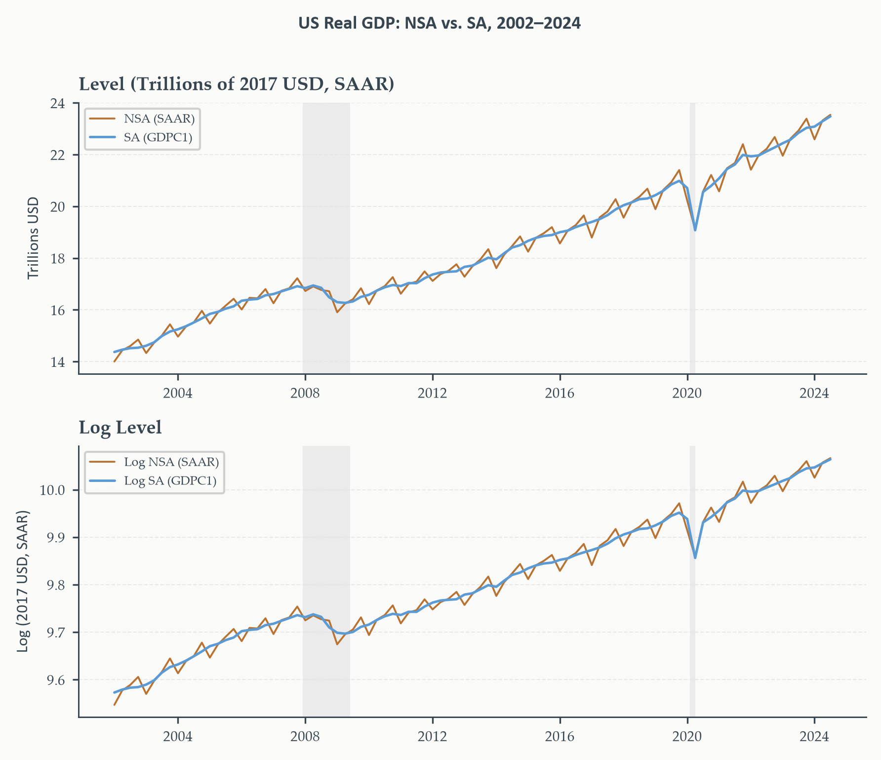
A note on units before we proceed. `GDPC1` — the official SA series — is published as a **Seasonally Adjusted Annual Rate** (SAAR): each quarterly observation is multiplied by four to express the economy's pace as if that quarter's output were sustained for a full year. `ND000334Q` is a quarterly *total*, not annualised. Plotting them in raw form would show the SA series running about four times higher than the NSA series — not because the economy is larger, but because the units differ. We convert the NSA quarterly totals to SAAR (multiply by 4) before plotting so that the two series are directly comparable.
```{python}
#| label: fig-gdp-nsa-sa
#| fig-cap: "US Real GDP: NSA (SAAR) vs. officially SA, from first available observation through 2024. Both series are expressed as seasonally adjusted annual rates (billions of 2017 USD) to ensure comparability — the raw NSA series is a quarterly total, while GDPC1 is already annualised. The NSA series (copper) exhibits pronounced intra-year oscillation around the SA trend (blue). On the log scale (bottom panel) the oscillations are proportionally stable over time, confirming that the multiplicative model — equivalently, the additive model on logs — is the appropriate decomposition framework."
#| fig-width: 6
#| fig-height: 5
#| code-fold: true
#| code-summary: "Show code — NSA vs SA real GDP"
fig, axes = plt.subplots(2, 1, figsize=(6, 5))

ax = axes[0]
ax.plot(gdp.index, gdp["Real GDP (NSA, SAAR)"] / 1e3, color=EO_COPPER,  lw=0.9, label="NSA (SAAR)")
ax.plot(gdp.index, gdp["Real GDP (SA)"]         / 1e3, color=EO_SKYBLUE, lw=1.2, label="SA (GDPC1)")
shade_recessions(ax, start=PLOT_START)
ax.set_title("Level (Trillions of 2017 USD, SAAR)")
ax.set_ylabel("Trillions USD")
ax.legend(loc="upper left")
eo_style_ax(ax)

ax = axes[1]
ax.plot(gdp.index, gdp["Log NSA"], color=EO_COPPER,  lw=0.9, label="Log NSA (SAAR)")
ax.plot(gdp.index, gdp["Log SA"],  color=EO_SKYBLUE, lw=1.2, label="Log SA (GDPC1)")
shade_recessions(ax, start=PLOT_START)
ax.set_title("Log Level")
ax.set_ylabel("Log (2017 USD, SAAR)")
ax.legend(loc="upper left")
eo_style_ax(ax)

end_yr = gdp.index[-1].year
eo_suptitle(fig, f"US Real GDP: NSA vs. SA, {gdp.index[0].year}–{end_yr}")
fig.tight_layout()
plt.show()
```
The figure makes the seasonal pattern visible. In levels, the NSA series oscillates around the SA trend with an amplitude that grows over time — the hallmark of a multiplicative seasonal pattern. In logs, the oscillations are proportionally stable, confirming our earlier reasoning. Going forward, we work primarily in log levels unless otherwise noted.
## Moving Averages {#sec-moving-averages}
### Trend Estimation by Moving Averages
The oldest and most transparent approach to trend estimation is the [moving average](https://en.wikipedia.org/wiki/Moving_average). The idea is as simple as it sounds: average out the short-run fluctuations by replacing each observation with a local average of the observations around it. Whatever remains after that local averaging is the trend. Whatever the trend misses is the seasonal and irregular.
For a quarterly series with period $m = 4$, the **centered moving average** of order 4 is:
$$\hat{T}_t = \frac{1}{8}\,y_{t-2} + \frac{1}{4}\,y_{t-1} + \frac{1}{4}\,y_t + \frac{1}{4}\,y_{t+1} + \frac{1}{8}\,y_{t+2}$$
Where do these weights come from? The $2 \times 4$-MA is built in two steps. First, compute a simple 4-term average centered half a period ahead of $t$:
$$M_t^+ = \tfrac{1}{4}(y_{t-1} + y_t + y_{t+1} + y_{t+2})$$
and another centered half a period behind:
$$M_t^- = \tfrac{1}{4}(y_{t-2} + y_{t-1} + y_t + y_{t+1})$$
Then average the two:
$$\hat{T}_t = \tfrac{1}{2}(M_t^+ + M_t^-) = \tfrac{1}{8}y_{t-2} + \tfrac{1}{4}y_{t-1} + \tfrac{1}{4}y_t + \tfrac{1}{4}y_{t+1} + \tfrac{1}{8}y_{t+2}$$
The second step — averaging $M_t^+$ and $M_t^-$ — is what makes the result exactly centered at $t$ and gives each of the four calendar quarters equal total weight of $\frac{1}{4}$. This equal-weight property is precisely what is needed to cancel a seasonal pattern with period 4: averaging over exactly one full year of quarters removes any fixed quarterly effect. For monthly data ($m = 12$), the analogous $2 \times 12$-MA follows the same logic.
::: {.callout-note}
## The Classical Decomposition Algorithm
Given a time series $\{y_t\}$ with seasonal period $m$:
1. **Estimate the trend** $\hat{T}_t$ using a centered $2 \times m$ moving average.
2. **Remove the trend**: compute de-trended observations $d_t = y_t - \hat{T}_t$ (additive) or $d_t = y_t / \hat{T}_t$ (multiplicative).
3. **Estimate seasonal factors** $\hat{S}_j$ for each period $j = 1, \ldots, m$ by averaging all de-trended values that fall in period $j$ across years:
$$\hat{S}_j^{\text{raw}} = \frac{1}{N_j}\sum_{t:\,\text{season}(t)=j} d_t$$
where $N_j$ is the number of years in which period $j$ appears. Normalize so that the seasonal factors sum to zero (additive) or average to one (multiplicative).
4. **Compute the irregular component**: $\hat{I}_t = y_t - \hat{T}_t - \hat{S}_t$ (additive) or $\hat{I}_t = y_t / (\hat{T}_t \cdot \hat{S}_t)$ (multiplicative).
Note that the moving average loses observations at both ends of the sample: $\lfloor m/2 \rfloor$ at the start and $\lfloor m/2 \rfloor$ at the end. This is a practical cost of all local-smoothing trend estimators.
:::
The moving average trend has an important limitation: it follows the data closely enough that it can absorb some of the business cycle variation we actually want to preserve in the irregular component. There is no free parameter to control the degree of smoothing — the window width is determined by the seasonal period. This is one of the reasons that more sophisticated trend filters, discussed in Section 2.3, have largely replaced simple moving averages in business cycle analysis, even while classical decomposition remains a useful first pass.
### Decomposing Log NSA GDP
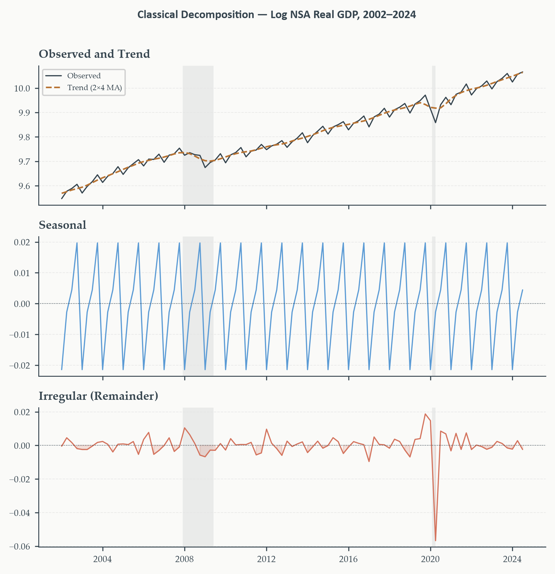
Let us apply classical decomposition to the log NSA GDP series using `statsmodels`. We use the multiplicative model (equivalently, additive on logs) with period $m = 4$.
```{python}
#| label: fig-classical-decomp
#| fig-cap: "Classical additive decomposition of log NSA real GDP. Top panel: observed log level (charcoal) overlaid with the 2×4 moving average trend (copper) — the overlap makes visible how closely the trend tracks the long-run path and where the seasonal and irregular components pull the data away from it. Middle panel: seasonal factors (four quarterly constants), stable across the postwar period and large relative to the irregular. Bottom panel: irregular remainder, the component that contains the business cycle signal. NBER recessions are shaded throughout."
#| fig-width: 6
#| fig-height: 6
#| code-fold: true
#| code-summary: "Show code — Classical decomposition"
decomp = seasonal_decompose(gdp["Log NSA"], model="additive", period=4, extrapolate_trend="freq")

fig, axes = plt.subplots(3, 1, figsize=(6, 6), sharex=True)

# Panel 1: observed + trend overlaid
ax = axes[0]
ax.plot(gdp.index, gdp["Log NSA"],    color=EO_CHARCOAL, lw=0.9, label="Observed")
ax.plot(decomp.trend.index, decomp.trend.values, color=EO_COPPER, lw=1.2, ls="--", label="Trend (2×4 MA)")
shade_recessions(ax, start=PLOT_START)
ax.set_title("Observed and Trend")
ax.legend(loc="upper left", fontsize=6)
eo_style_ax(ax)

# Panel 2: seasonal
ax = axes[1]
ax.plot(decomp.seasonal.index, decomp.seasonal.values, color=EO_SKYBLUE, lw=0.9)
ax.axhline(0, color=EO_CHARCOAL, lw=0.5, ls=":")
shade_recessions(ax, start=PLOT_START)
ax.set_title("Seasonal")
eo_style_ax(ax)

# Panel 3: irregular
ax = axes[2]
ax.plot(decomp.resid.index, decomp.resid.values, color=EO_TERRACOTTA, lw=0.9)
ax.axhline(0, color=EO_CHARCOAL, lw=0.5, ls=":")
ax.fill_between(decomp.resid.index, decomp.resid.values, 0,
                where=(decomp.resid.values < 0), color=EO_TERRACOTTA, alpha=0.2)
shade_recessions(ax, start=PLOT_START)
ax.set_title("Irregular (Remainder)")
axes[-1].set_xlabel("")
eo_style_ax(ax)

end_yr = gdp.index[-1].year
eo_suptitle(fig, f"Classical Decomposition — Log NSA Real GDP, {gdp.index[0].year}–{end_yr}")
fig.tight_layout()
plt.show()
```
The trend is smooth and nearly linear in logs — consistent with the balanced growth path that growth theory predicts for a modern economy. The seasonal factors are large, swinging roughly $\pm 2$–$3\%$ relative to trend within each year, and they are strikingly stable across the postwar period: the same quarterly rhythm repeating for nearly eighty years. That stability is precisely what justifies the fixed-factor assumption embedded in classical decomposition, and it is the signal that seasonal adjustment is designed to strip away. What remains in the irregular component is noisy but economically meaningful — clear recessionary dips are visible at 1974–75, 1981–82, 2008–09, and 2020, all corresponding to NBER-dated recessions. Throughout, all components are in log units: a seasonal factor of $+0.02$, for example, means output is approximately $2\%$ above its trend value in that quarter.
### From Moving Averages to Linear Filters
The irregular from a classical decomposition is our first, crude estimate of the business cycle. It is crude for two reasons. The moving average trend absorbs some cyclical variation, making cycles appear smaller than they are. And the fixed seasonal factors assume the seasonal pattern never changes, which may be unrealistic over very long samples. Section 2.3 develops better tools for trend extraction, and Section 2.5 addresses the seasonal component more carefully.
The deeper limitation is that there is no optimization involved. The number of periods to average is fixed by the seasonal period, the weights are fixed by the two-step construction, and there is no smooth adjustment as the trend evolves. Section 2.3 introduces the linear filter family, which replaces these fixed conventions with a minimization problem — finding the smoothest trend that still tracks the data.
## Linear Filters {#sec-linear-filters}
### Linear and Quadratic Detrending
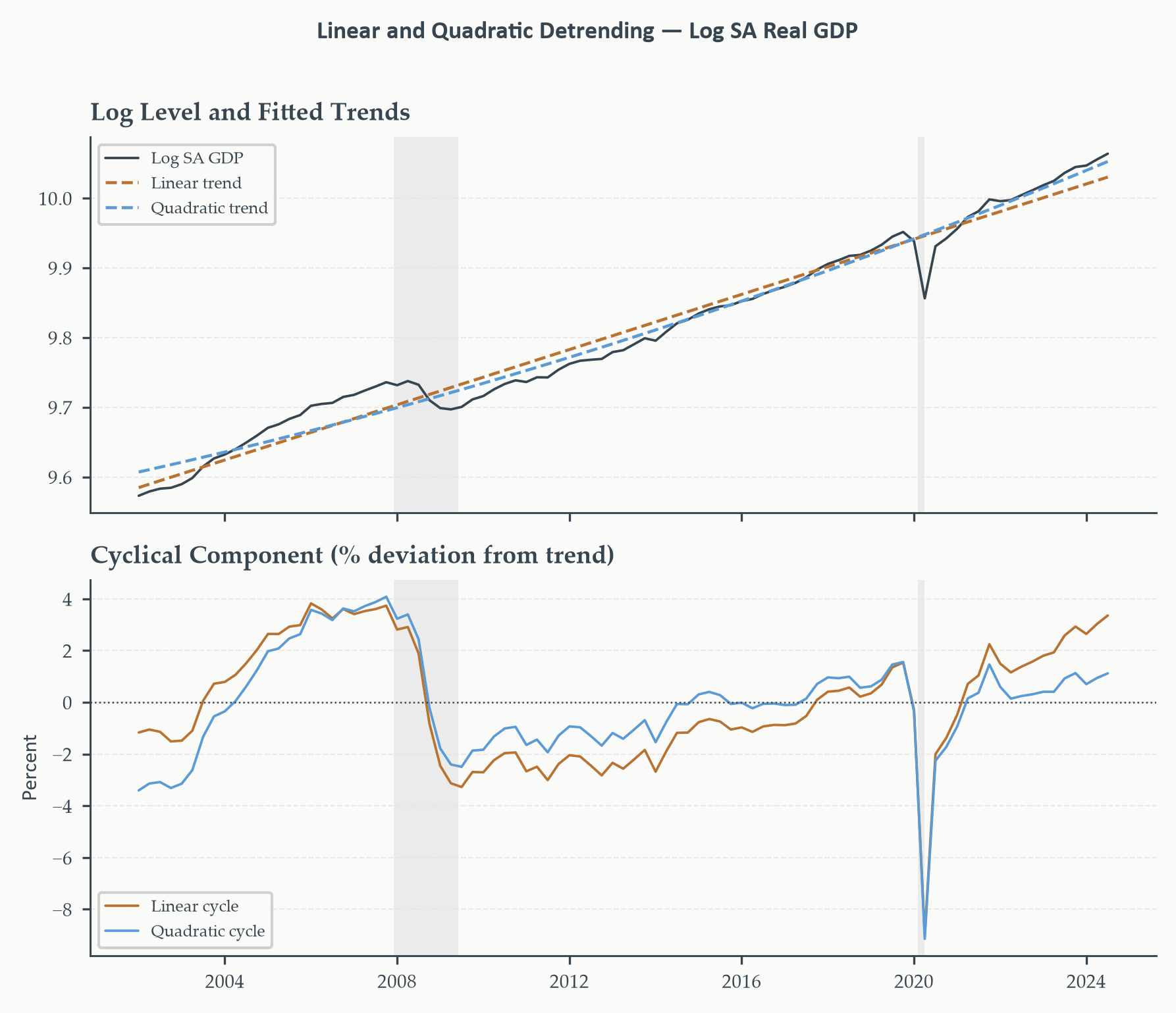
The simplest possible linear filter asks: what if the trend is just a straight line? We assume the log of output grows at a constant rate over time, and any deviation from that line is cyclical. This is the **linear detrending** approach. We estimate it by regressing log GDP on a linear time index $t$:
$$\log y_t = \alpha + \beta t + \varepsilon_t \tag{2.1}$$
The OLS regression finds the line $\hat{\alpha} + \hat{\beta} t$ that best fits the log series in a least-squares sense. The residual $\hat{\varepsilon}_t = \log y_t - \hat{\alpha} - \hat{\beta} t$ is the cyclical component — the percentage deviation of output from its estimated linear trend.
A natural extension allows for a changing growth rate by including a quadratic term:
$$\log y_t = \alpha + \beta t + \gamma t^2 + \varepsilon_t \tag{2.2}$$
The quadratic trend can accommodate the well-documented postwar productivity slowdown — the fact that US potential output appears to have grown faster in the 1950s–60s than in the decades since.
Both approaches embed a strong assumption: that the trend is purely deterministic. Shocks to output are transitory — the economy always reverts to the same fixed path. We found evidence in Chapter 1 that log real GDP is $I(1)$: its unit root means shocks are at least partly permanent. Imposing a deterministic trend on a unit-root process is a form of misspecification. The trend will chase the data, and the extracted cycle will be contaminated by whatever the trend misses. Still, as a simple first pass — and as a baseline against which richer methods can be compared — linear and quadratic detrending are worth knowing.
```{python}
#| label: fig-linear-detrend
#| fig-cap: "Linear and quadratic detrending of log SA real GDP. Top panel: the log level with both fitted trends. Bottom panel: the cyclical components (residuals). The linear trend forces US output to revert to a single long-run growth rate, making the 1970s slowdown appear as an extended negative cycle and the 1990s boom appear as a substantial positive one. The quadratic trend captures the productivity slowdown by allowing the growth rate to change, shifting the extracted cycle. NBER recession dates are shaded in both panels."
#| fig-width: 6
#| fig-height: 5
#| code-fold: true
#| code-summary: "Show code — Linear and quadratic detrending"
log_sa = gdp["Log SA"].dropna()
T      = len(log_sa)
t      = np.arange(1, T + 1)

# OLS detrending
X_lin  = np.column_stack([np.ones(T), t])
X_quad = np.column_stack([np.ones(T), t, t**2])

b_lin  = np.linalg.lstsq(X_lin,  log_sa.values, rcond=None)[0]
b_quad = np.linalg.lstsq(X_quad, log_sa.values, rcond=None)[0]

trend_lin  = X_lin  @ b_lin
trend_quad = X_quad @ b_quad

cycle_lin  = log_sa.values - trend_lin
cycle_quad = log_sa.values - trend_quad

fig, axes = plt.subplots(2, 1, figsize=(6, 5), sharex=True)

ax = axes[0]
ax.plot(log_sa.index, log_sa.values,  color=EO_CHARCOAL,   lw=0.9, label="Log SA GDP")
ax.plot(log_sa.index, trend_lin,       color=EO_COPPER,     lw=1.1, ls="--", label="Linear trend")
ax.plot(log_sa.index, trend_quad,      color=EO_SKYBLUE,    lw=1.1, ls="--", label="Quadratic trend")
shade_recessions(ax, start=PLOT_START)
ax.set_title("Log Level and Fitted Trends")
ax.legend(loc="upper left", fontsize=6)
eo_style_ax(ax)

ax = axes[1]
ax.plot(log_sa.index, cycle_lin  * 100, color=EO_COPPER,  lw=0.9, label="Linear cycle")
ax.plot(log_sa.index, cycle_quad * 100, color=EO_SKYBLUE, lw=0.9, label="Quadratic cycle")
ax.axhline(0, color=EO_CHARCOAL, lw=0.6, ls=":")
shade_recessions(ax, start=PLOT_START)
ax.set_title("Cyclical Component (% deviation from trend)")
ax.set_ylabel("Percent")
ax.legend(loc="lower left", fontsize=6)
eo_style_ax(ax)

eo_suptitle(fig, "Linear and Quadratic Detrending — Log SA Real GDP")
fig.tight_layout()
plt.show()
```
The bottom panel illustrates the dependence problem clearly. The choice of trend determines the cycle. The linear trend, by forcing a single constant growth rate on the entire postwar period, interprets the 1970s as a sustained negative deviation and the late 1990s as a large positive one. The quadratic trend, by allowing the growth rate itself to change, recalibrates both episodes. Neither is wrong in a technical sense — both minimize least squares on their respective parameterizations — but they tell quite different stories about the economy's cyclical position at any given date.
### The HP Filter
By far the most widely used tool for business cycle extraction in macroeconomics is the **[Hodrick-Prescott filter](https://en.wikipedia.org/wiki/Hodrick%E2%80%93Prescott_filter)**, introduced in a 1980 working paper ([published in 1997](https://www.kellogg.northwestern.edu/research/math/papers/451.pdf)). Its central appeal is that it solves a transparent optimization problem: find a smooth trend that tracks the data without following every wiggle.
Formally, given a time series $\{y_t\}_{t=1}^T$, the HP filter finds the trend $\{\tau_t\}$ that minimizes:
$$\sum_{t=1}^{T}(y_t - \tau_t)^2 + \lambda \sum_{t=2}^{T-1}\bigl[(\tau_{t+1} - \tau_t) - (\tau_t - \tau_{t-1})\bigr]^2 \tag{2.3}$$
The first sum penalizes deviations of the trend from the data — it pushes the trend toward the series. The second sum penalizes changes in the growth rate of the trend — it pushes the trend toward a straight line. The scalar $\lambda > 0$ governs the trade-off between these two objectives.
::: {.callout-note}
## Definition 2.2 — The HP Filter
The **Hodrick-Prescott filter** extracts a trend $\{\hat{\tau}_t\}$ from $\{y_t\}$ by solving:
$$\min_{\{\tau_t\}} \left\{ \sum_{t=1}^{T}(y_t - \tau_t)^2 + \lambda \sum_{t=2}^{T-1}\bigl[(\tau_{t+1} - \tau_t) - (\tau_t - \tau_{t-1})\bigr]^2 \right\}$$
The smoothing parameter $\lambda$ controls the flexibility of the trend. As $\lambda \to 0$, the trend passes through every data point (no smoothing). As $\lambda \to \infty$, the trend approaches a straight line (maximum smoothing). The conventional choices, due to Hodrick and Prescott, are $\lambda = 1600$ for quarterly data, $\lambda = 14400$ for monthly data, and $\lambda = 100$ for annual data.
The cyclical component is defined as $\hat{c}_t = y_t - \hat{\tau}_t$.
:::
The second term in the objective penalizes $(\tau_{t+1} - \tau_t) - (\tau_t - \tau_{t-1})$, which is the second difference of the trend — the change-in-change, or discrete approximation to the second derivative. Penalizing this means the filter resists trends that accelerate or decelerate rapidly. The solution to the optimization problem is linear in $y$ and can be written in matrix form as $\hat{\tau} = (I + \lambda K'K)^{-1} y$, where $K$ is the $(T-2) \times T$ second-difference matrix. In practice, `statsmodels.tsa.filters.hp_filter.hpfilter` computes this for us.
The HP filter became the de facto standard in the business cycle literature — used in hundreds of empirical papers, taught in every graduate macroeconomics course — because it is simple to apply, transparent in its objective, and produces cycles that broadly match the NBER recession dates. But it has also attracted serious criticism, most forcefully from James Hamilton.
### Hamilton's Critique and Alternative
In a [2018 paper](https://direct.mit.edu/rest/article-abstract/100/5/831/58479/Why-You-Should-Never-Use-the-Hodrick-Prescott?redirectedFrom=fulltext) in the *Review of Economics and Statistics*, James Hamilton argued that the HP filter has three fundamental problems that render its output unreliable for business cycle analysis.
First, the HP filter generates spurious cycles even when the true data-generating process has none. Hamilton showed that applying the HP filter to a pure random walk — a process with no cyclical component by construction — produces a cyclical residual with the same statistical properties as what practitioners report as business cycles. The filter manufactures structure from noise.
Second, the HP filter produces substantial **end-point bias**: the trend estimate near the most recent observations is especially sensitive to the choice of $\lambda$, because the filter has less data on one side to anchor the trend. In real-time applications — precisely when policymakers need reliable estimates — the HP cycle is least trustworthy.
Third, the second-difference penalty implicitly assumes the trend is integrated of order two ($I(2)$). But log real GDP is $I(1)$, not $I(2)$. The HP filter is solving the right optimization problem for the wrong class of process.
**Hamilton's alternative** is disarmingly simple. He proposes projecting $y_{t+h}$ on the four most recent values of $y$:
$$y_{t+h} = \beta_0 + \beta_1 y_t + \beta_2 y_{t-1} + \beta_3 y_{t-2} + \beta_4 y_{t-3} + \varepsilon_{t+h} \tag{2.4}$$
and using the OLS residual as the cyclical component. For quarterly GDP, Hamilton recommends $h = 8$ (two years ahead). The residual $\hat{\varepsilon}_{t+h}$ captures the part of $y_{t+h}$ that is not predictable from the recent history of the series. To see why this is a natural cycle measure: if output is highly persistent, the best prediction of where it will be in two years is simply where it is today. Anything that diverges from that prediction — unexpectedly high or low output relative to its own recent trend — is the cyclical component. The residual is not noise; it is the surprise, and surprises relative to the trend path are exactly what the business cycle measures.
This approach has several advantages over HP. It is robust to the order of integration of $y_t$ — it works whether the series is $I(1)$ or trend-stationary. It has no end-point bias, since both ends of the sample lose observations symmetrically. It does not require choosing a smoothing parameter. And it does not generate spurious cycles from noise.
The main disadvantage is interpretive: the Hamilton filter extracts a cycle at the frequency $1/h$, which for $h = 8$ quarters corresponds to a two-year horizon. This is somewhat shorter than the conventional NBER business cycle, and it misses lower-frequency variation that the HP filter would retain. As with every decomposition choice, this is a feature — Hamilton's filter is asking a specific question — but one that users should be aware of.
### The HP Filter's End-Point Problem: A Policy Illustration
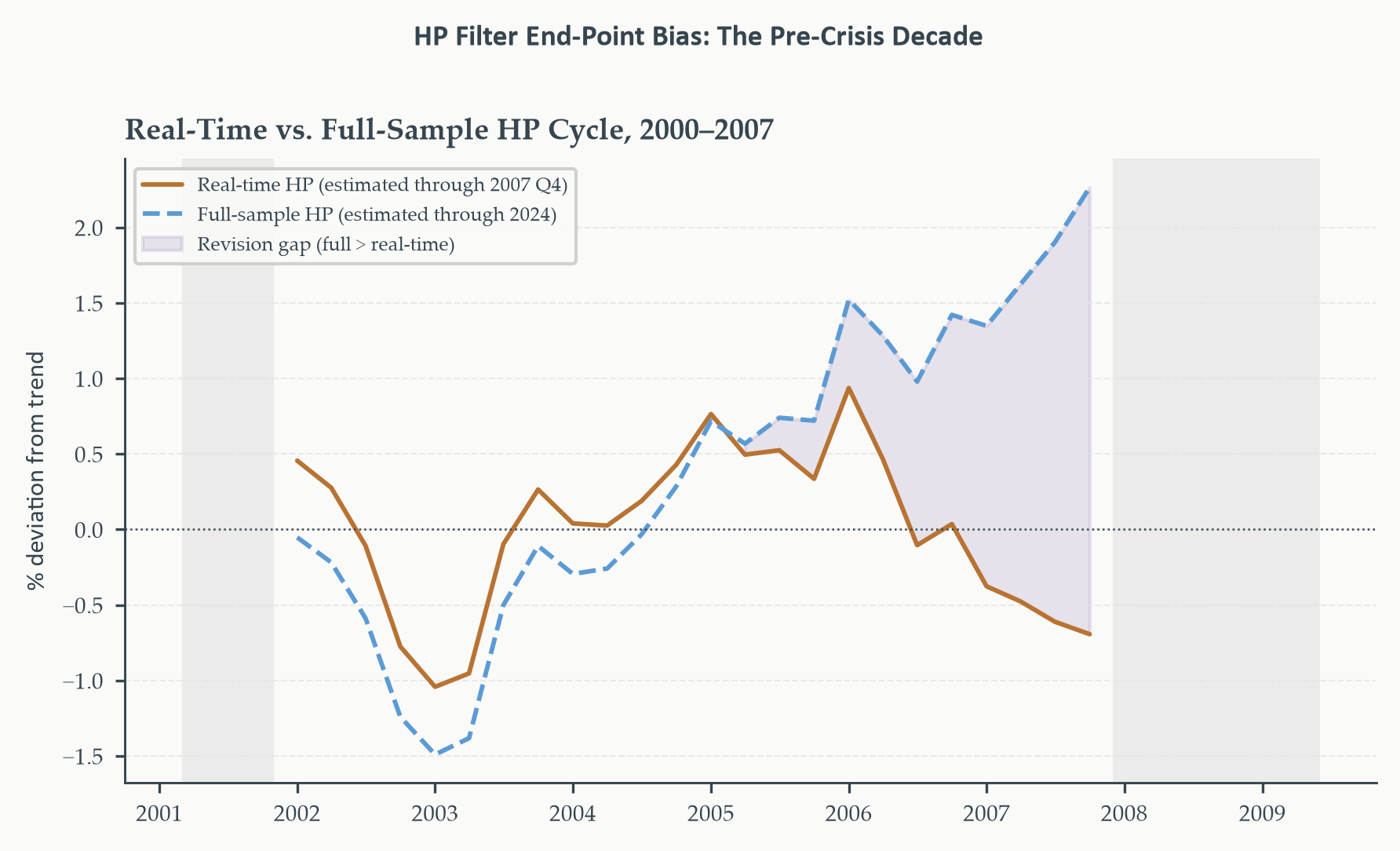
The end-point bias of the HP filter is not merely a statistical curiosity. It can lead a policymaker who relies on real-time HP estimates to draw the opposite conclusion from the one the data, in hindsight, support. The pre-2008 period offers a vivid illustration.
Run the HP filter on log SA real GDP using only data available through 2007 Q4 — the last quarter before the financial crisis was officially dated as having begun. The HP trend, fitted on data that ends at the peak of a long expansion, has no future observations to pull it down. It therefore interprets a substantial portion of the 2004–2007 growth as trend rather than cycle. The result: a modest positive cycle, perhaps $+1$ to $+2\%$. The economy looks roughly at potential. A policymaker reading this in early 2008 might conclude no major policy response is needed.
Now run the same HP filter on data through 2024. The Great Recession and its protracted recovery are now in the sample. The filter's trend for 2007 is pulled *down* relative to the real-time estimate — with a deep trough visible after 2008, the filter places the pre-crisis trend lower, which makes the pre-crisis deviation from trend larger. The 2007 cycle in the full-sample HP estimate is substantially more positive: perhaps $+3$ to $+4\%$. In hindsight, the economy was running considerably hotter than the real-time filter suggested.
```{python}
#| label: fig-hp-endpoint
#| fig-cap: "HP filter end-point bias over the pre-crisis decade, 2000–2007. Both lines use λ=1600 on the same log SA real GDP series. The copper line is the HP cycle a policymaker would have seen in real time, estimated on data through 2007 Q4 only. The blue dashed line is the full-sample cycle estimated on data through 2024. Near the 2007 peak the real-time cycle (copper) is close to zero or modestly positive, while the full-sample cycle (blue dashed) is clearly and persistently above it. The lavender band marks the revision gap where the full-sample estimate exceeds the real-time estimate — consistently positive every year of the expansion."
#| fig-width: 6
#| fig-height: 3.5
#| code-fold: true
#| code-summary: "Show code — HP end-point bias"
log_sa_full = gdp["Log SA"].dropna()

cutoff     = "2007-10-01"   # data through 2007 Q4
zoom_start = "2000-01-01"

# Real-time HP: estimated on data up to cutoff only
log_sa_rt        = log_sa_full[log_sa_full.index <= cutoff]
cycle_hp_rt, _   = hpfilter(log_sa_rt, lamb=1600)

# Full-sample HP
cycle_hp_full, trend_hp = hpfilter(log_sa_full, lamb=1600)
cycle_hp_full_sub = cycle_hp_full[cycle_hp_full.index <= cutoff]

# Zoom both series to 2000–2007 for clarity
rt_zoom   = cycle_hp_rt[cycle_hp_rt.index >= zoom_start]
full_zoom = cycle_hp_full_sub[cycle_hp_full_sub.index >= zoom_start]

fig, ax = plt.subplots(figsize=(6, 3.5))

ax.plot(rt_zoom.index,   rt_zoom.values * 100,
        color=EO_COPPER,  lw=1.4, label="Real-time HP (estimated through 2007 Q4)")
ax.plot(full_zoom.index, full_zoom.values * 100,
        color=EO_SKYBLUE, lw=1.4, ls="--", label="Full-sample HP (estimated through 2024)")
ax.axhline(0, color=EO_CHARCOAL, lw=0.6, ls=":")
ax.fill_between(rt_zoom.index,
                rt_zoom.values * 100,
                full_zoom.values * 100,
                where=(full_zoom.values >= rt_zoom.values),
                alpha=0.18, color=EO_LAVENDER, label="Revision gap (full > real-time)")
shade_recessions(ax, start=zoom_start, end="2009-06-01")
ax.set_title("Real-Time vs. Full-Sample HP Cycle, 2000–2007")
ax.set_ylabel("% deviation from trend")
ax.legend(loc="upper left", fontsize=6)
eo_style_ax(ax)
eo_suptitle(fig, "HP Filter End-Point Bias: The Pre-Crisis Decade")
fig.tight_layout()
plt.show()
```
The lavender band is the revision gap — consistently positive across 2004–2007, meaning the real-time filter understated the boom in every single year of the pre-crisis expansion. A central bank relying on the real-time HP cycle would have seen a roughly neutral output gap and moderate tightening at most; the full-sample estimate reveals an economy running substantially above potential. End-point bias is not random noise: it is systematic, it is worst near the frontier of the data, and it biases the cycle toward zero precisely when policymakers most need an accurate read.
This is the policy consequence of end-point bias. The Hamilton filter, by construction, does not have this property. Its cycle estimate at any date $t$ depends only on observations available well before $t$ (since the residual is dated $t+h$ and uses data from $t$ backward), so the real-time and full-sample estimates coincide.
## Exponential Smoothing {#sec-ses}
Moving averages and linear filters approach decomposition retrospectively: given the full series, extract components by filtering or regression. Exponential smoothing takes a different starting point — the forecasting problem. The question it answers is: given a stream of observations arriving one at a time, how should we update our estimate of the current level of the series as each new observation arrives?
The insight is that recent observations should count for more than old ones. An observation from last quarter is more informative about where the economy is right now than an observation from ten years ago. But the observation from ten years ago should not be thrown away entirely — it contains some information, just less. Exponential smoothing formalizes this intuition by assigning geometrically declining weights to past observations.
### Simple Exponential Smoothing
**[Simple exponential smoothing](https://en.wikipedia.org/wiki/Exponential_smoothing)** (SES) is designed for series with no trend and no seasonality — a level that fluctuates around a slowly moving mean. The smoothed level at time $t$ is:
$$\hat{y}_{t+1|t} = \alpha y_t + (1 - \alpha)\hat{y}_{t|t-1} \tag{2.5}$$
where $\alpha \in (0,1)$ is the **smoothing parameter**. The forecast for the next period is a weighted blend of the current observation $y_t$ and last period's forecast $\hat{y}_{t|t-1}$.
Expanding the recursion reveals why this is called exponential smoothing:
$$\hat{y}_{t+1|t} = \alpha y_t + \alpha(1-\alpha)y_{t-1} + \alpha(1-\alpha)^2 y_{t-2} + \cdots$$
The weight on observation $y_{t-k}$ is $\alpha(1-\alpha)^k$, which declines geometrically in $k$. A small $\alpha$ (close to zero) places heavy weight on old observations: the smoothed level changes slowly and the forecast is nearly a long-run average. A large $\alpha$ (close to one) places almost all weight on the most recent observation: the forecast tracks the data closely and reacts quickly to new information.
::: {.callout-note}
## Definition 2.3 — Simple Exponential Smoothing
Given observations $y_1, \ldots, y_T$ and a smoothing parameter $\alpha \in (0,1)$, the **SES** forecast is:
$$\hat{y}_{t+1|t} = \alpha y_t + (1-\alpha)\hat{y}_{t|t-1}, \quad t = 1, 2, \ldots, T$$
initialized at $\hat{y}_{1|0} = y_1$ (or estimated as a free parameter). The $h$-step-ahead forecast is flat: $\hat{y}_{T+h|T} = \hat{y}_{T+1|T}$ for all $h \geq 1$. SES is appropriate for series with no trend and no seasonality.
:::
An equivalent and illuminating way to write equation (2.5) is the **error-correction form**:
$$\hat{y}_{t+1|t} = \hat{y}_{t|t-1} + \alpha e_t, \qquad e_t = y_t - \hat{y}_{t|t-1}$$
where $e_t$ is the one-step forecast error. Each new forecast adjusts the previous forecast by a fraction $\alpha$ of the most recent error. Large $\alpha$ means aggressive updating; small $\alpha$ means conservative updating.
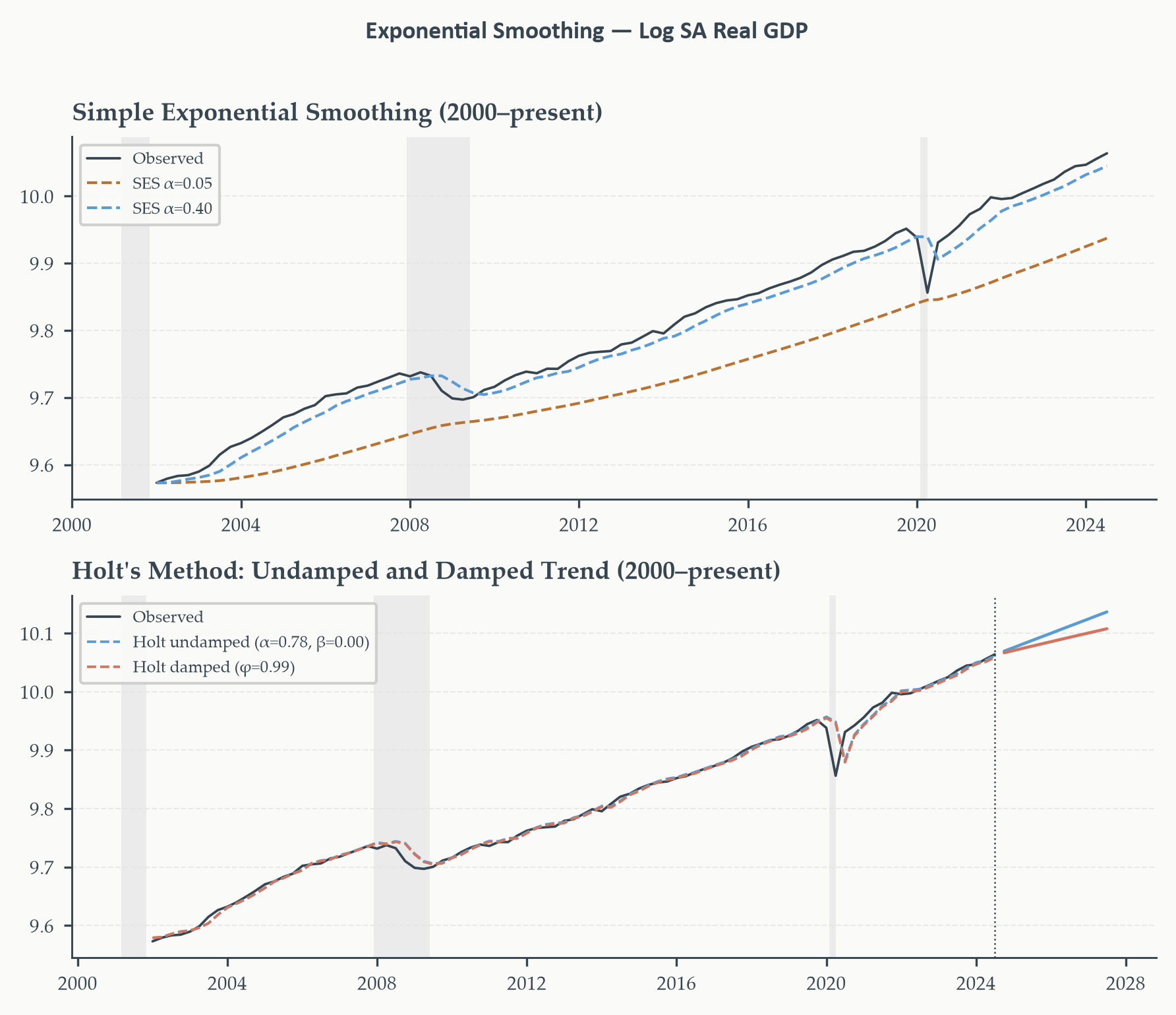
SES produces **flat** multi-step forecasts: since there is no trend in the model, the best forecast at any horizon $h \geq 1$ is the current smoothed level. This is appropriate for stationary series, but for trending series like GDP we need to extend the framework.
### Holt's Method: Adding a Trend
**[Holt's linear exponential smoothing](https://en.wikipedia.org/wiki/Exponential_smoothing#Double_exponential_smoothing_(Holt_linear))** extends SES by maintaining a separate smoothed estimate of the trend alongside the level. The equations are:
$$\hat{\ell}_t = \alpha y_t + (1-\alpha)(\hat{\ell}_{t-1} + \hat{b}_{t-1}) \tag{2.6}$$
$$\hat{b}_t = \beta(\hat{\ell}_t - \hat{\ell}_{t-1}) + (1-\beta)\hat{b}_{t-1} \tag{2.7}$$
$$\hat{y}_{t+h|t} = \hat{\ell}_t + h\hat{b}_t \tag{2.8}$$
Here $\hat{\ell}_t$ is the smoothed level and $\hat{b}_t$ is the smoothed trend (slope). Equation (2.6) updates the level as a blend of the new observation and a one-step-ahead forecast from the previous state. Equation (2.7) updates the trend as a blend of the current change in level and the previous trend estimate. The $h$-step-ahead forecast (2.8) projects the current level forward at the current slope.
An important variant is **Holt's damped trend method**, which multiplies the trend by a damping factor $\phi \in (0,1)$ at each forecast horizon:
$$\hat{y}_{t+h|t} = \hat{\ell}_t + (\phi + \phi^2 + \cdots + \phi^h)\hat{b}_t$$
For large $h$, the cumulative factor $\sum_{i=1}^h \phi^i \to \phi/(1-\phi)$ as $h \to \infty$, so the long-run forecast approaches a finite level rather than growing without bound. Empirical evidence consistently shows that damped trend forecasts outperform undamped ones at medium and long horizons.
```{python}
#| label: fig-ses-holt
#| fig-cap: "Simple exponential smoothing (top) and Holt's method with and without damping (bottom), applied to the log SA real GDP series. SES with small α produces a smooth level that lags the trending data considerably; larger α tracks the data more closely. Holt's method extrapolates the recent slope linearly (blue) or with damping (terracotta), which flattens at longer horizons. Parameters are estimated by maximum likelihood."
#| fig-width: 6
#| fig-height: 5
#| code-fold: true
#| code-summary: "Show code — SES and Holt's method"
# Use the officially SA series — STL-SA is computed later in Section 2.5
series_fit = gdp["Log SA"].dropna()

ses_low  = SimpleExpSmoothing(series_fit).fit(smoothing_level=0.05, optimized=False)
ses_high = SimpleExpSmoothing(series_fit).fit(smoothing_level=0.4,  optimized=False)

holt_und = Holt(series_fit).fit(optimized=True)
holt_dmp = Holt(series_fit, damped_trend=True).fit(optimized=True)

h_fcast  = 12
ses_start = "2000-01-01"
s = series_fit[series_fit.index >= ses_start]

fig, axes = plt.subplots(2, 1, figsize=(6, 5), sharex=False)

# ── SES panel ─────────────────────────────────────────────────────────────────
ax = axes[0]
ax.plot(s.index, s.values, color=EO_CHARCOAL, lw=0.9, label="Observed")
ax.plot(s.index, ses_low.fittedvalues[ses_low.fittedvalues.index >= ses_start],
        color=EO_COPPER, lw=1.0, ls="--", label="SES α=0.05")
ax.plot(s.index, ses_high.fittedvalues[ses_high.fittedvalues.index >= ses_start],
        color=EO_SKYBLUE, lw=1.0, ls="--", label="SES α=0.40")
shade_recessions(ax, start=ses_start)
ax.set_title("Simple Exponential Smoothing (2000–present)")
ax.legend(loc="upper left", fontsize=6)
eo_style_ax(ax)

# ── Holt panel ────────────────────────────────────────────────────────────────
ax = axes[1]
last_date = series_fit.index[-1]
fcast_idx = pd.date_range(last_date, periods=h_fcast + 1, freq="QS")[1:]
fcast_und = holt_und.forecast(h_fcast)
fcast_dmp = holt_dmp.forecast(h_fcast)

ax.plot(s.index, s.values, color=EO_CHARCOAL, lw=0.9, label="Observed")
ax.plot(s.index, holt_und.fittedvalues[holt_und.fittedvalues.index >= ses_start],
        color=EO_SKYBLUE, lw=0.9, ls="--",
        label=f"Holt undamped (α={holt_und.params['smoothing_level']:.2f}, β={holt_und.params['smoothing_trend']:.2f})")
ax.plot(s.index, holt_dmp.fittedvalues[holt_dmp.fittedvalues.index >= ses_start],
        color=EO_TERRACOTTA, lw=0.9, ls="--",
        label=f"Holt damped (φ={holt_dmp.params['damping_trend']:.2f})")
ax.plot(fcast_idx, fcast_und.values, color=EO_SKYBLUE,    lw=1.1, ls="-")
ax.plot(fcast_idx, fcast_dmp.values, color=EO_TERRACOTTA, lw=1.1, ls="-")
ax.axvline(last_date, color=EO_CHARCOAL, lw=0.6, ls=":")
shade_recessions(ax, start=ses_start)
ax.set_title("Holt's Method: Undamped and Damped Trend (2000–present)")
ax.legend(loc="upper left", fontsize=6)
eo_style_ax(ax)

eo_suptitle(fig, "Exponential Smoothing — Log SA Real GDP")
fig.tight_layout()
plt.show()
```
The figure illustrates the key behavioral difference between the two methods. SES produces a smooth level that works well for series without trend, but it systematically lags a trending series — it is always trying to catch up. Holt's method follows the trend by construction. The undamped forecast extrapolates the recent slope linearly and diverges from the damped version over longer horizons. For a series as persistently trending as GDP, the damped version is almost always more appropriate: it is skeptical that the most recently estimated growth rate will persist indefinitely.
### The ETS Framework
The exponential smoothing methods developed so far can be organized into a unified framework known as **ETS** — named for its three components: **E**rror, **T**rend, and **S**easonality. This framework, developed formally by Hyndman et al. ([2002](https://www.sciencedirect.com/science/article/pii/S0169207001001108), [2008](https://link.springer.com/book/10.1007/978-3-540-71918-2)), provides a systematic taxonomy of all sensible combinations of exponential smoothing components, along with a formal statistical model — with likelihood function and prediction intervals — for each combination.
Each of the three components can take different forms:
- **Error (E):** additive (A) or multiplicative (M)
- **Trend (T):** none (N), additive (A), additive damped (Ad), multiplicative (M), multiplicative damped (Md)
- **Seasonality (S):** none (N), additive (A), multiplicative (M)
The notation ETS(E,T,S) identifies a specific model. ETS(A,N,N) is simple exponential smoothing with additive errors — the SES model above. ETS(A,A,N) is Holt's undamped linear method. ETS(A,Ad,N) is Holt's damped method. The Holt-Winters seasonal models are ETS(A,A,A) and ETS(A,A,M).
The four cases that matter most in macroeconomic applications are:
**ETS(A,N,N) — Simple Exponential Smoothing.** No trend, no seasonality, additive error. The level equation is $\hat{\ell}_t = \hat{\ell}_{t-1} + \alpha e_t$ where $e_t = y_t - \hat{\ell}_{t-1}$ is the one-step forecast error. (Here and throughout the key-cases descriptions we write $e_t$ as shorthand for the error at time $t$; the dependence on the parameter vector $\theta$ through the state recursion is implicit, and made explicit in the MLE discussion below.) Forecasts are flat. Appropriate for stationary or slowly-drifting series with no seasonal pattern.
**ETS(A,A,N) — Holt's Linear Method.** Additive trend, no seasonality, additive error. Level and slope both updated each period. Forecasts follow a linear projection from the current state. The undamped version extrapolates linearly; caution is warranted at long horizons.
**ETS(A,Ad,N) — Holt's Damped Method.** Additive damped trend, no seasonality. Forecasts converge to a finite level as $h \to \infty$. Empirically, this is often the single best-performing exponential smoothing model across a wide range of real datasets, particularly at medium horizons.
**ETS(A,A,A) — Holt-Winters Additive.** Additive trend, additive seasonal, additive error. Appropriate when the series has been log-transformed, so that multiplicative seasonality in levels becomes additive seasonality in logs.
::: {.callout-note}
## Definition 2.4 — The Holt-Winters Additive Model: ETS(A,A,A)
Given a seasonal period $m$, the state equations are:
$$\hat{\ell}_t = \alpha(y_t - \hat{s}_{t-m}) + (1-\alpha)(\hat{\ell}_{t-1} + \hat{b}_{t-1}) \tag{2.9}$$
$$\hat{b}_t = \beta(\hat{\ell}_t - \hat{\ell}_{t-1}) + (1-\beta)\hat{b}_{t-1} \tag{2.10}$$
$$\hat{s}_t = \gamma(y_t - \hat{\ell}_{t-1} - \hat{b}_{t-1}) + (1-\gamma)\hat{s}_{t-m} \tag{2.11}$$
$$\hat{y}_{t+h|t} = \hat{\ell}_t + h\hat{b}_t + \hat{s}_{t+h-m(k+1)} \tag{2.12}$$
where $k = \lfloor (h-1)/m \rfloor$ ensures the correct seasonal index is used, and $\gamma \in (0, 1-\alpha)$ is the seasonal smoothing parameter. Three smoothing parameters — $\alpha$, $\beta$, $\gamma$ — and the initial states $\{\hat{\ell}_0, \hat{b}_0, \hat{s}_{1-m}, \ldots, \hat{s}_0\}$ are estimated jointly by maximum likelihood.
The **damped variant, ETS(A,Ad,A)**, replaces $h\hat{b}_t$ in equation (2.12) with $\left(\sum_{i=1}^h \phi^i\right)\hat{b}_t$, where $\phi \in (0,1)$ is the damping parameter. Forecasts converge to a finite level as $h \to \infty$ rather than extrapolating the trend linearly. We fit the damped version in the Python example below, as it is almost always preferred at longer forecast horizons.
:::
The three smoothing equations have a parallel structure. The level (2.9) is updated as a blend of the de-seasonalized observation $y_t - \hat{s}_{t-m}$ and the extrapolated level from the previous state. The trend (2.10) updates the slope. The seasonal factor (2.11) updates the seasonal index for period $t$ as a blend of the de-trended observation and the same-season factor from one full year ago. The forecast (2.12) adds the projected level, the projected trend, and the appropriate seasonal factor.
The full ETS framework extends to 30 combinations by allowing multiplicative errors and multiplicative seasonality, each with its own state equations and likelihood function. For log-transformed series the additive variants are almost always appropriate. Readers interested in the complete taxonomy will find it in Hyndman et al. (2008), *Forecasting with Exponential Smoothing: The State Space Approach*.
### Parameter Estimation and Forecasting
Parameters in ETS models — the smoothing parameters $\alpha$, $\beta$, $\gamma$, $\phi$ and the initial states — are estimated by **[maximum likelihood](https://en.wikipedia.org/wiki/Maximum_likelihood_estimation)**. Let $\theta$ collect all parameters. The one-step-ahead forecast errors are computed recursively as $e_t(\theta) = y_t - \hat{y}_{t|t-1}(\theta)$. Under Gaussian errors, profiling out $\sigma^2$ gives the **concentrated log-likelihood**:
$$\ell_c(\theta) = -\frac{T}{2}\left[1 + \log(2\pi) + \log\hat{\sigma}^2(\theta)\right], \qquad \hat{\sigma}^2(\theta) = \frac{1}{T}\sum_{t=1}^T e_t(\theta)^2$$
Maximizing $\ell_c(\theta)$ is equivalent to minimizing $\sum e_t(\theta)^2$. The advantage of full MLE is that initial states are estimated as free parameters rather than set by convention, and the likelihood supports model comparison via AIC.
With parameters estimated, point forecasts follow from running the state equations forward from the end of the sample. [Prediction intervals](https://en.wikipedia.org/wiki/Prediction_interval) are computed by simulation: draw future innovation sequences, propagate them through the state equations, and take empirical quantiles. These intervals widen with horizon — appropriately capturing the fact that uncertainty compounds as we look further ahead. Prediction intervals **are not** [confidence intervals](https://en.wikipedia.org/wiki/Confidence_interval): they account for future forecast uncertainty, not parameter uncertainty, so in practice they will be slightly too narrow.
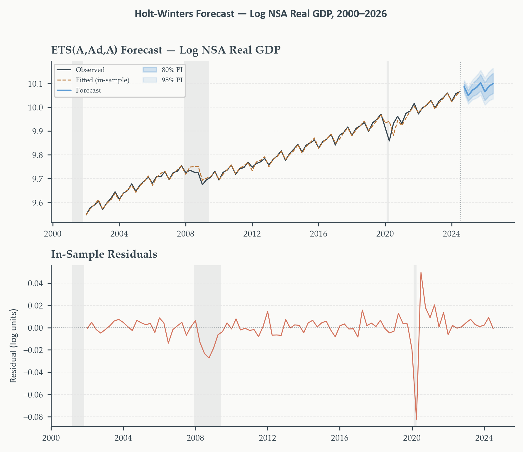
```{python}
#| label: fig-hw-forecast
#| fig-cap: "Holt-Winters ETS(A,Ad,A) forecast for log NSA real GDP, 2000–2026. The model is fit on the full available sample and forecasts eight quarters ahead. The seasonal pattern is extrapolated from the estimated seasonal factors; the damped trend reflects appropriate skepticism about the persistence of the recent growth rate. The 80% and 95% prediction intervals (shaded bands) widen with horizon. NBER recessions are shaded; the sharp 2020 outlier is visible in the residuals."
#| fig-width: 6
#| fig-height: 5
#| code-fold: true
#| code-summary: "Show code — Holt-Winters forecast"
series_nsa = gdp["Log NSA"].dropna()

hw_model = ExponentialSmoothing(
    series_nsa,
    trend="add",
    damped_trend=True,
    seasonal="add",
    seasonal_periods=4,
    initialization_method="estimated",
).fit(optimized=True)

h_ahead  = 8
fcast    = hw_model.forecast(h_ahead)

sim      = hw_model.simulate(h_ahead, repetitions=5000, error="add")
pi_80_lo = np.percentile(sim, 10, axis=1)
pi_80_hi = np.percentile(sim, 90, axis=1)
pi_95_lo = np.percentile(sim, 2.5, axis=1)
pi_95_hi = np.percentile(sim, 97.5, axis=1)

fcast_idx = fcast.index
hw_start  = "2000-01-01"

fig, axes = plt.subplots(2, 1, figsize=(6, 5))

ax = axes[0]
obs_plot = series_nsa[series_nsa.index >= hw_start]
ax.plot(obs_plot.index, obs_plot.values, color=EO_CHARCOAL, lw=0.9, label="Observed")
ax.plot(hw_model.fittedvalues[hw_model.fittedvalues.index >= hw_start].index,
        hw_model.fittedvalues[hw_model.fittedvalues.index >= hw_start].values,
        color=EO_COPPER, lw=0.8, ls="--", label="Fitted (in-sample)")
ax.plot(fcast_idx, fcast.values, color=EO_SKYBLUE, lw=1.2, label="Forecast")
ax.fill_between(fcast_idx, pi_80_lo, pi_80_hi, color=EO_SKYBLUE, alpha=0.25, label="80% PI")
ax.fill_between(fcast_idx, pi_95_lo, pi_95_hi, color=EO_SKYBLUE, alpha=0.12, label="95% PI")
ax.axvline(series_nsa.index[-1], color=EO_CHARCOAL, lw=0.6, ls=":")
shade_recessions(ax, start=hw_start)
ax.set_title("ETS(A,Ad,A) Forecast — Log NSA Real GDP")
ax.legend(loc="upper left", fontsize=5.5, ncol=2)
eo_style_ax(ax)

ax = axes[1]
resid_plot = hw_model.resid[hw_model.resid.index >= hw_start]
ax.plot(resid_plot.index, resid_plot.values, color=EO_TERRACOTTA, lw=0.8)
ax.axhline(0, color=EO_CHARCOAL, lw=0.6, ls=":")
shade_recessions(ax, start=hw_start)
ax.set_title("In-Sample Residuals")
ax.set_ylabel("Residual (log units)")
eo_style_ax(ax)

print(f"Fitted parameters:")
print(f"  α (level):    {hw_model.params['smoothing_level']:.4f}")
print(f"  β (trend):    {hw_model.params['smoothing_trend']:.4f}")
print(f"  γ (seasonal): {hw_model.params['smoothing_seasonal']:.4f}")
print(f"  φ (damping):  {hw_model.params['damping_trend']:.4f}")
print(f"  AIC:          {hw_model.aic:.2f}")
print(f"  BIC:          {hw_model.bic:.2f}")

end_yr = fcast_idx[-1].year
eo_suptitle(fig, f"Holt-Winters Forecast — Log NSA Real GDP, 2000–{end_yr}")
fig.tight_layout()
plt.show()
```
The level smoothing parameter $\alpha$ reflects how quickly the model updates its estimate of the current level in response to new observations. The damping parameter $\phi$ (close to 1 but below it) indicates modest damping — the model retains most of the trend momentum but expects it to fade somewhat over the forecast horizon. The seasonal parameter $\gamma$ controls how much the model learns about seasonal factors from each new year of data. The 2020 Q2 observation produces a large negative residual — COVID-19, an exogenous shock outside the information set of any statistical model. This is a reflection of the model's appropriate ignorance about regime-changing events, not evidence of misspecification. Even from this single in-sample fit, the seasonal structure, trend momentum, and interval widths give us the key ingredients for the evaluation exercise in Chapter 5 — where we will ask not just whether the forecasts look reasonable, but whether they beat a benchmark and how their uncertainty is calibrated. A full framework for out-of-sample evaluation — including rolling windows, the Diebold-Mariano test, and forecast combination — is developed there.
## Seasonal Adjustment in Practice {#sec-seasonal}
Seasonal patterns in economic data are large, predictable, and economically uninteresting — which is exactly what makes them dangerous. A policymaker looking at raw retail sales in January would see a sharp drop from December every single year, regardless of underlying economic conditions. A central bank reacting to every seasonal swing in the unemployment rate would be setting monetary policy in response to noise. Seasonal adjustment strips out these predictable rhythms so that the signal — the underlying trend and cycle — is easier to see.
Most official economic statistics are reported in seasonally adjusted form as the default. The employment situation report, the GDP advance estimate, industrial production, new housing starts — all are seasonally adjusted before publication. The methodology behind those adjustments matters because it shapes the data that researchers, forecasters, and policymakers use every day.
### X-13-ARIMA-SEATS: The Government's Method
The US Bureau of Economic Analysis, Bureau of Labor Statistics, and statistical agencies across most developed economies adjust their data using **[X-13-ARIMA-SEATS](https://www.census.gov/data/software/x13as.html)**, a software package maintained by the US Census Bureau. Understanding what it does — even without running it — is essential for interpreting official statistics.
X-13 is the current generation of a lineage that began with the X-11 program developed at the Census Bureau in 1965. The original X-11 was a pure iterative moving-average filter — no ARIMA, no model-based decomposition. It evolved through X-11-ARIMA (Statistics Canada, 1980), which added ARIMA-based endpoint extension; X-12-ARIMA (Census Bureau, 1998), which expanded the ARIMA specification tools and diagnostics; and finally X-13-ARIMA-SEATS (2012), which added SEATS as a fully model-based alternative to the iterative filter. When analysts and texts refer to "the X-11 filter," they mean the iterative moving-average procedure that originated in 1965 and is still used as the core method inside X-13 today — X-11 names both the original standalone program and the inherited filter component.
Understanding the procedure in sequence makes its logic clear.
::: {.callout-note}
## How X-13-ARIMA-SEATS Works: Step by Step
**Step 1 — ARIMA extension.** Fit an ARIMA model to the raw series and use it to extend the series one to three years forward (and optionally backward). This gives the filter data at both ends of the sample, solving the endpoint loss problem that afflicts classical decomposition and the HP filter. (Chapter 3 covers ARIMA models in full.)
**Step 2 — Prior adjustment.** Remove known deterministic effects before filtering: trading day variation (the number of Mondays, Tuesdays, … in each month varies), holiday effects (Easter, Thanksgiving), and outliers flagged by automatic detection. These are modelled as regression effects and subtracted from the extended series.
**Step 3 — X-11 filter (iterative moving averages).** Apply a sequence of moving averages to the prior-adjusted, extended series:
- Estimate a preliminary trend using a long moving average.
- Subtract the trend to isolate the combined seasonal and irregular.
- Average across years by season to obtain preliminary seasonal factors.
- Subtract the seasonal factors to get a preliminary seasonally adjusted series.
- Re-estimate the trend on this cleaner series; repeat the cycle.
After two or three passes, the estimates converge. At each pass, outlier weights are updated to reduce the influence of extreme observations. The result is a smooth, stable set of seasonal factors that are allowed to evolve slowly over time.
**Step 4 — Discard the extensions.** Drop the ARIMA-forecasted values added in Step 1. The final seasonal factors and seasonally adjusted series cover only the original sample.
**Step 4 (alternative) — SEATS instead of the X-11 filter.** Rather than applying the iterative moving-average filter in Step 3, the SEATS method (Signal Extraction in ARIMA Time Series) uses the ARIMA model from Step 1 to perform a model-based canonical decomposition. It allocates the spectrum of the series mathematically across trend, seasonal, and irregular components. SEATS has a firmer statistical foundation than the X-11 filter and tends to produce smoother seasonal factors; it is the method of choice in most European statistical agencies and is increasingly preferred in the US as well.
:::
Why does X-13 require a dedicated binary rather than a simple Python function? Because the procedure above — particularly the prior adjustment for trading days and holidays, the automatic ARIMA specification search, the outlier detection logic, and the diagnostic suite — represents decades of accumulated refinements in production-grade Fortran code. The `statsmodels` library provides a Python wrapper (`statsmodels.tsa.x13.x13_arima_analysis`) that calls the X-13 binary, but the binary itself must be installed separately from the Census Bureau website. For research and teaching purposes the methods we implement directly in Python are sufficient and considerably more transparent; for producing official statistics, X-13 is the unavoidable standard.
### STL Decomposition: A Flexible, Portable Alternative
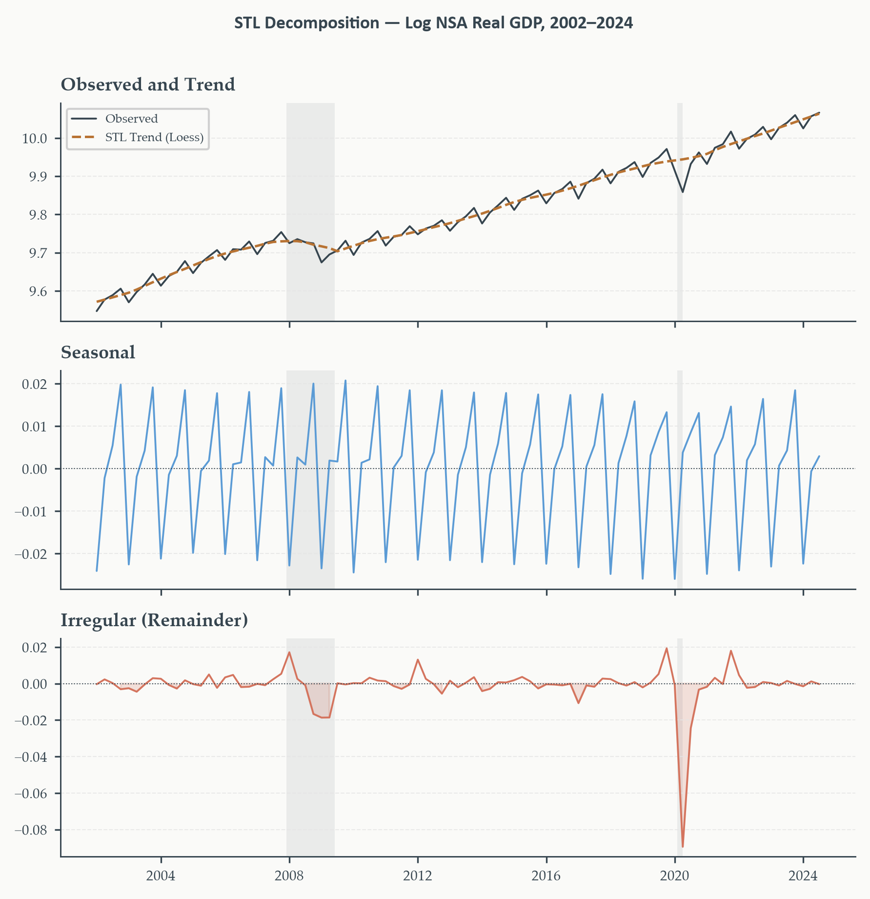
The method we will use for seasonal decomposition is **STL** — Seasonal-Trend decomposition using Loess — introduced by [Cleveland et al. (1990)](https://www.scb.se/contentassets/ca21efb41fee47d293bbee5bf7be7fb3/stl-a-seasonal-trend-decomposition-procedure-based-on-loess.pdf). STL is implemented natively in `statsmodels` without any external binary dependency, it is highly flexible, and it handles many of the practical challenges that classical decomposition cannot.
STL is an iterative procedure. It alternates between two passes: an inner loop that updates the seasonal and trend estimates given the current decomposition, and an outer loop that computes robustness weights to reduce the influence of outliers. The trend at each step is estimated using **Loess** (locally weighted polynomial regression), which fits a low-degree polynomial to a local neighborhood of the data at each point — more flexible than a global moving average and less prone to distortion near structural shifts.
The main differences from X-13 are worth stating clearly. STL treats the seasonal component as slowly varying but does not model calendar effects (trading day counts, Easter, holidays). X-13 explicitly adjusts for these. STL is additive by default (or multiplicative on logs). X-13 integrates ARIMA-based forecasting to avoid end-point loss. STL is fully transparent and implemented in Python; X-13 is an institutional production standard with decades of accumulated refinements. For research and teaching, STL is the right tool. For producing the official figures that appear in a statistical release, X-13 is the standard.
```{python}
#| label: fig-stl-decomp
#| fig-cap: "STL decomposition of log NSA real GDP. Top panel: observed log level overlaid with the STL Loess trend — the trend is smoother and more flexible than the classical moving average, adapting to the productivity slowdown of the 1970s and the post-2008 recovery. Middle panel: seasonal component, allowed to evolve slowly over time. Bottom panel: irregular remainder, the component that contains the business cycle signal."
#| fig-width: 6
#| fig-height: 6
#| code-fold: true
#| code-summary: "Show code — STL decomposition"
stl    = STL(gdp["Log NSA"], period=4, seasonal=7, robust=True)
result = stl.fit()

# STL seasonal-adjusted series — used in comparisons below
gdp["Log STL-SA"] = gdp["Log NSA"] - result.seasonal

fig, axes = plt.subplots(3, 1, figsize=(6, 6), sharex=True)

ax = axes[0]
ax.plot(gdp.index, gdp["Log NSA"],   color=EO_CHARCOAL, lw=0.9, label="Observed")
ax.plot(result.trend.index, result.trend.values, color=EO_COPPER, lw=1.2, ls="--", label="STL Trend (Loess)")
shade_recessions(ax, start=PLOT_START)
ax.set_title("Observed and Trend")
ax.legend(loc="upper left", fontsize=6)
eo_style_ax(ax)

ax = axes[1]
ax.plot(result.seasonal.index, result.seasonal.values, color=EO_SKYBLUE, lw=0.9)
ax.axhline(0, color=EO_CHARCOAL, lw=0.5, ls=":")
shade_recessions(ax, start=PLOT_START)
ax.set_title("Seasonal")
eo_style_ax(ax)

ax = axes[2]
ax.plot(result.resid.index, result.resid.values, color=EO_TERRACOTTA, lw=0.9)
ax.axhline(0, color=EO_CHARCOAL, lw=0.5, ls=":")
ax.fill_between(result.resid.index, result.resid.values, 0,
                where=(result.resid.values < 0), color=EO_TERRACOTTA, alpha=0.2)
shade_recessions(ax, start=PLOT_START)
ax.set_title("Irregular (Remainder)")
axes[-1].set_xlabel("")
eo_style_ax(ax)

end_yr = gdp.index[-1].year
eo_suptitle(fig, f"STL Decomposition — Log NSA Real GDP, {gdp.index[0].year}–{end_yr}")
fig.tight_layout()
plt.show()
```
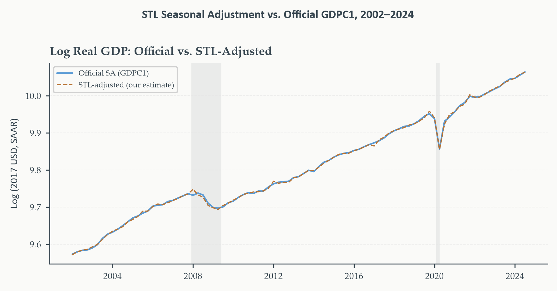
```{python}
#| label: fig-stl-vs-official
#| fig-cap: "Comparison of STL-adjusted and officially SA real GDP. The STL adjustment (copper dashed) closely tracks the BEA's X-13-based SA series (blue), with the two differing primarily in periods of structural change (post-2008, post-2020) where X-13's ARIMA-based end-extension and calendar adjustment provide marginally smoother estimates. The correspondence is close enough for research and teaching purposes."
#| fig-width: 6
#| fig-height: 3
#| code-fold: true
#| code-summary: "Show code — STL vs official SA comparison"
fig, ax = plt.subplots(figsize=(6, 3))
ax.plot(gdp.index, gdp["Log SA"],
        color=EO_SKYBLUE, lw=1.2, label="Official SA (GDPC1)")
ax.plot(gdp.index, gdp["Log STL-SA"],
        color=EO_COPPER, lw=0.9, ls="--", label="STL-adjusted (our estimate)")
shade_recessions(ax, start=PLOT_START)
ax.set_title("Log Real GDP: Official vs. STL-Adjusted")
ax.set_ylabel("Log (2017 USD, SAAR)")
ax.legend(loc="upper left")
eo_style_ax(ax)
end_yr = gdp.index[-1].year
eo_suptitle(fig, f"STL Seasonal Adjustment vs. Official GDPC1, {gdp.index[0].year}–{end_yr}")
fig.tight_layout()
plt.show()
```
The correspondence between the STL-adjusted series and the official SA series is close — close enough to validate the approach for our purposes. The differences are largest in the most recent quarters and around the major structural breaks (2008–09, 2020), exactly where X-13's ARIMA pre-extension and calendar adjustment provide the most additional precision.
### What Seasonal Adjustment Removes — and What It Does Not
It is worth being precise about what seasonal adjustment actually does to the data. It removes the component of variation that is systematic and calendar-driven — the predictable swings associated with the time of year. It does not remove all short-run volatility; the irregular component survives. It does not smooth out recessions; a recession that hits hardest in Q4 will still appear as a sharp decline in the adjusted series, even if Q4 is normally a strong quarter.
One practical implication: seasonal adjustment can interact with structural change in ways that produce artifacts. If the 2020 pandemic caused an unprecedented collapse in Q2 — far outside the range of historical Q2 observations — then seasonal adjustment algorithms estimated on pre-pandemic data will temporarily misestimate the seasonal factor for Q2 in subsequent years. This is why the BLS and BEA issued multiple revisions to seasonal factors in 2020–2022 and why analysts following real-time data always need to be aware of the vintage of seasonal factors being applied.
## What Is the Business Cycle? {#sec-biz-cycle}
### Deviations from Trend
The [business cycle](https://en.wikipedia.org/wiki/Business_cycle) is one of the most studied and debated concepts in macroeconomics, yet it is surprisingly hard to define precisely. The phrase conjures images of booms and busts, expansions and recessions, the rhythmic up-and-down of economic activity. But this intuitive picture conceals a fundamental ambiguity: up and down relative to what?
If we mean relative to last period, we are looking at growth rates — and growth rates are always fluctuating, even in a healthy economy. If we mean relative to a fixed level, we have the problem that the economy trends upward over time and never returns to its past level. The only economically coherent benchmark is the trend — the economy's long-run potential path — and deviations from that trend are what we mean by the business cycle:
$$\hat{I}_t = y_t - \hat{T}_t - \hat{S}_t$$
This definition has an important implication: the business cycle is not a natural object sitting in the data waiting to be discovered. It is a residual — what is left after we remove the trend and seasonal components. And because different methods produce different trends, they produce different business cycles. This is not a methodological embarrassment; it is an economically meaningful fact. Whether the 1990s boom appears large or modest, whether the 2001 recession looks shallow or deep, depends directly on how we model the trend that GDP is deviating from.
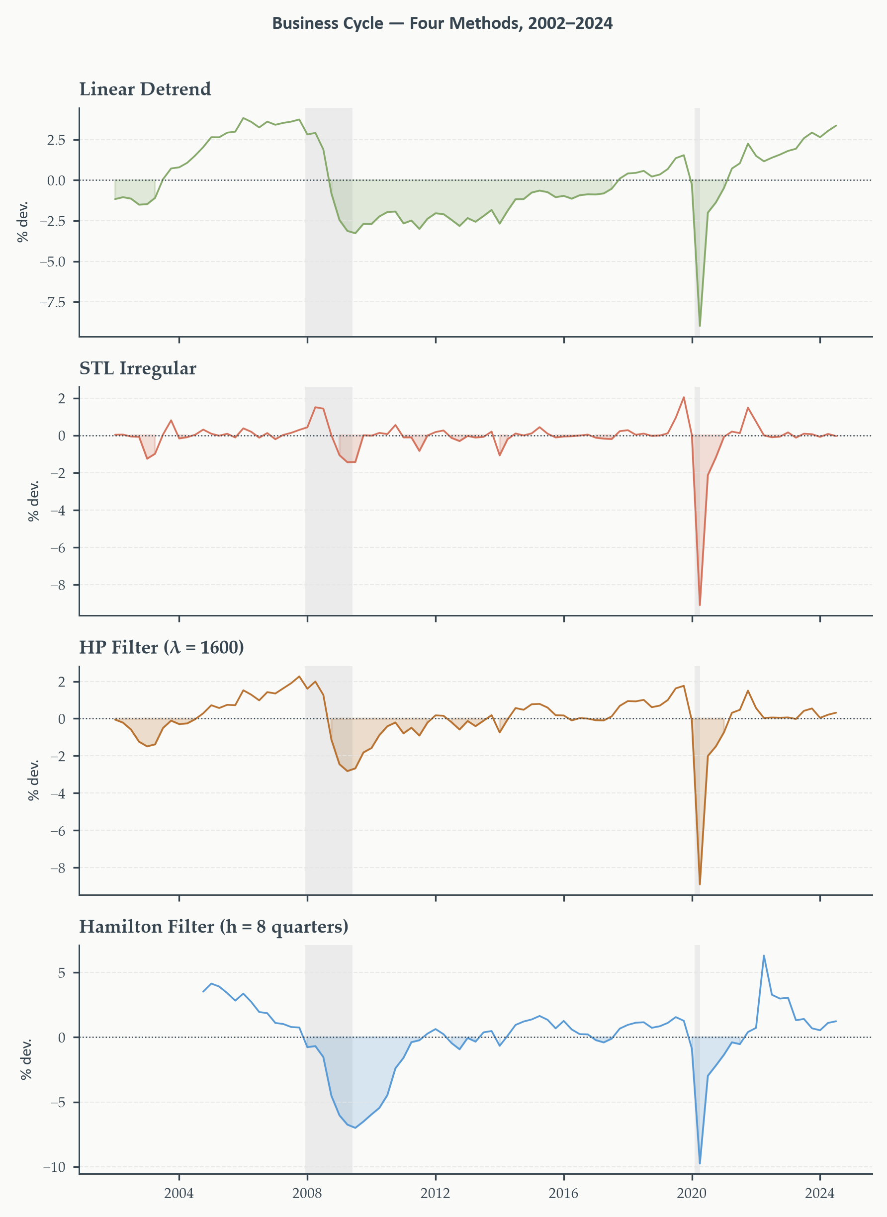
We have now developed four methods for extracting a cycle, and we can compare them directly. The figure below plots each method's cycle on the same time axis. With all four methods in hand, the comparison is fair — the reader knows exactly what each panel is showing and why.
```{python}
#| label: fig-biz-cycle-comparison
#| fig-cap: "Business cycle components from four methods applied to log SA real GDP, ordered as introduced in this chapter. Top: linear detrend (sage). Second: STL irregular (terracotta) — the least opinionated method, retaining the most high-frequency variation because it imposes no smoothing bandwidth, penalty parameter, or projection horizon. Third: HP filter (λ=1600, copper). Bottom: Hamilton filter (h=8 quarters, blue). NBER recessions are shaded throughout. The Hamilton panel is blank for the first several quarters by construction: the filter requires h=8 quarters of lead time plus four lags, so the first residual is only available once those observations accumulate — an honest acknowledgement of the method's data requirements, and the reason it has no end-point bias."
#| fig-width: 6
#| fig-height: 8
#| code-fold: true
#| code-summary: "Show code — Four-method cycle comparison"
log_sa_full = gdp["Log SA"].dropna()

# ── HP Filter ─────────────────────────────────────────────────────────────────
cycle_hp, _ = hpfilter(log_sa_full, lamb=1600)

# ── Hamilton Filter ────────────────────────────────────────────────────────────
h_ham = 8
lags  = 4
y_arr = log_sa_full.values
n     = len(y_arr)

t_start = lags - 1
t_end   = n - 1 - h_ham

dep  = y_arr[(t_start + h_ham):(t_end + h_ham + 1)]
regs = np.column_stack([
    np.ones(len(dep)),
    y_arr[t_start:t_end + 1],
    y_arr[t_start - 1:t_end],
    y_arr[t_start - 2:t_end - 1],
    y_arr[t_start - 3:t_end - 2],
])
b_ham   = np.linalg.lstsq(regs, dep, rcond=None)[0]
resid   = dep - regs @ b_ham

ham_dates = log_sa_full.index[(t_start + h_ham):(t_end + h_ham + 1)]
cycle_ham = pd.Series(resid, index=ham_dates)

# ── STL Irregular (on SA series for fair comparison) ──────────────────────────
stl_sa    = STL(log_sa_full, period=4, seasonal=7, robust=True).fit()
cycle_stl = pd.Series(stl_sa.resid, index=log_sa_full.index)

# ── Linear detrend cycle (computed in Section 2.3) ────────────────────────────
cycle_lin_s = pd.Series(cycle_lin, index=log_sa_full.index)

# ── Plot ───────────────────────────────────────────────────────────────────────
labels = [
    "Linear Detrend",
    "STL Irregular",
    "HP Filter (λ = 1600)",
    "Hamilton Filter (h = 8 quarters)",
]
cycles = [cycle_lin_s * 100, cycle_stl * 100, cycle_hp * 100, cycle_ham * 100]
colors = [EO_SAGE, EO_TERRACOTTA, EO_COPPER, EO_SKYBLUE]

fig, axes = plt.subplots(4, 1, figsize=(6, 8), sharex=True)

for ax, cyc, label, color in zip(axes, cycles, labels, colors):
    ax.plot(cyc.index, cyc.values, color=color, lw=0.85)
    ax.axhline(0, color=EO_CHARCOAL, lw=0.6, ls=":")
    ax.fill_between(cyc.index, cyc.values, 0,
                    where=(cyc.values < 0),
                    color=color, alpha=0.22)
    shade_recessions(ax, start=PLOT_START)
    ax.set_title(label)
    ax.set_ylabel("% dev.")
    eo_style_ax(ax)

end_yr = gdp.index[-1].year
eo_suptitle(fig, f"Business Cycle — Four Methods, {gdp.index[0].year}–{end_yr}")
fig.tight_layout()
plt.show()
```
The four-panel figure rewards careful reading. All four methods identify the same major recessions — the 1974–75, 1981–82, 2008–09, and 2020 downturns are clearly negative in every panel. But they disagree substantially on the level, amplitude, and timing of cycles between recessions.
The **linear detrend** cycle is the most volatile of the smooth methods. By constraining the trend to a single straight line fitted over the entire postwar period, it forces every deviation from that line — including the entire productivity slowdown of the 1970s — into the cyclical component. The result is a large, persistent negative cycle through the 1970s and a correspondingly large positive cycle through the late 1990s that almost certainly overstates the boom.
The **STL irregular** is the least opinionated series in the figure. Because STL's Loess trend is highly flexible and its seasonal factors are estimated rather than imposed, the remainder retains genuine high-frequency variation without having been smoothed by any bandwidth parameter or regression horizon. The other three cycles look smoother because they have imposed additional structure — a penalty parameter $\lambda$, a projection horizon $h$, or a global regression line — before the cycle is even extracted. STL imposes the least, so it shows the most. When it disagrees with HP or Hamilton, the disagreement is informative: it identifies variation that the smoother methods have absorbed into their trend rather than left in the cycle.
The **HP filter** produces the smoothest cycle. Its trend adapts continuously to the data, which is its strength and its weakness simultaneously. Near the end of the sample the HP cycle tends to be smaller in absolute value than the other methods — end-point bias in action, as we saw in Section 2.3.
The **Hamilton filter** panel is blank for the first several quarters. This is not a programming error — it is an honest feature of the method. The filter requires $h = 8$ quarters of lead time plus four lags, so the first residual is only available once those observations exist. Both ends of the sample lose observations symmetrically, which is exactly why the filter has no end-point bias.
### The Lucas Critique Connection
There is a deeper issue here that connects back to Chapter 1. Every detrending method embeds a structural assumption about the economy's long-run path: the HP filter assumes potential output is $I(2)$, Hamilton's filter assumes the cycle is unpredictable at a two-year horizon, linear detrending assumes a constant growth rate. When policymakers use a cycle estimate derived from one of these methods to calibrate a policy rule — raising rates when the output gap exceeds a threshold, for example — they are conditioning policy on a model of the trend. But as [Lucas (1976)](https://www.sciencedirect.com/science/article/pii/S0167223176800023) argued, agents observe and respond to policy, and their responses alter the statistical relationships on which the model was estimated. A trend estimated from pre-policy data may not be the right benchmark once the policy rule is in place.
The business cycle, in other words, is real — the economy genuinely expands and contracts — but its precise shape and magnitude are decomposition-dependent. When you read that the output gap is currently $+1.5\%$ or $-2\%$, you are reading a number that depends heavily on choices that rarely appear in the headline, and that is itself subject to the Lucas critique once it enters the policymaker's reaction function.
## Looking Ahead
The decomposition and smoothing methods in this chapter are intuitive and practically useful, but they rest on assumptions that Chapter 3 will justify — and in some cases tighten.
Chapter 3 develops the ARMA family of models, which provide the theoretical foundation for the methods introduced here. Simple exponential smoothing turns out to be the optimal forecast for an ARIMA(0,1,1) process; Holt's linear method corresponds to ARIMA(0,2,2); the Holt-Winters seasonal model corresponds to a seasonal ARIMA. These are not coincidences — the entire ETS family sits inside the ARIMA family as a set of restricted special cases. Understanding that connection unlocks better tools for model selection, residual diagnostics, and the construction of prediction intervals. It also connects the trend-cycle question from this chapter to a model-based answer: the Beveridge-Nelson decomposition, developed in Chapter 3, uses the estimated ARIMA structure of a series to separate its permanent and transitory components — a model-based answer to the same trend-cycle separation problem we approached statistically here, with no free smoothing parameter and a cycle uniquely pinned down by the estimated ARIMA model.
Chapter 6 addresses a limitation implicit throughout this chapter: all our methods assume the data-generating process is stable over the sample. If the trend growth rate of GDP changed structurally — as it did in the early 1970s productivity slowdown, and arguably again after 2008 — then a single HP filter or Holt-Winters model estimated over the full sample will fit neither regime well. Structural break tests, and the methods for handling them, belong to Chapter 6.
Chapter 5 provides the formal framework for evaluating the forecasts produced in this chapter. The Diebold-Mariano test asks whether two competing forecasts have statistically different accuracy. Forecast combination — averaging ETS with ARIMA with HP-based projections — often outperforms any individual method. And proper calibration of prediction intervals requires checking their empirical coverage over rolling windows.
## Key Terms
::: {.callout-note icon=false}
## Glossary
**Decomposition** — The representation of a time series as a combination of trend, seasonal, and irregular components. Additive: $y_t = T_t + S_t + I_t$. Multiplicative: $y_t = T_t \times S_t \times I_t$, equivalent to additive on logarithms.
**Trend** $T_t$ — The slow-moving, long-run level of a time series, abstracting from seasonal and irregular fluctuations.
**Seasonal component** $S_t$ — Systematic, calendar-driven fluctuations that repeat with fixed periodicity $m$ (4 for quarterly, 12 for monthly data).
**Irregular component** $I_t$ — The residual after trend and seasonal variation are removed; in macroeconomics, the component that contains the business cycle signal.
**Classical decomposition** — Trend estimation via a centered $2 \times m$ moving average, followed by averaging de-trended observations by season to estimate fixed seasonal factors.
**Linear filter** — A transformation of a time series that expresses each output value as a linear combination of input values. Moving averages, the HP filter, and OLS detrending are all linear filters; they differ in how they weight observations across the sample.
**HP filter** — The Hodrick-Prescott filter; extracts a smooth trend by minimizing a penalized sum of squares balancing fit against smoothness, governed by $\lambda$. Conventional choices: $\lambda = 1600$ (quarterly), $\lambda = 14400$ (monthly).
**Hamilton filter** — A regression-based cycle filter: project $y_{t+h}$ on four lags of $y_t$; the residual is the cycle. Avoids the spurious cycle generation and end-point bias problems of the HP filter.
**End-point bias** — The tendency of two-sided filters (including HP) to produce unreliable trend estimates near the ends of the sample, where the filter has less data on one side to anchor the trend. Worst in real-time applications.
**Business cycle** — The deviation of real output from its trend (potential) path. Not a natural object in the data, but a residual whose shape depends on the decomposition chosen.
**Output gap** — The percentage deviation of actual GDP from potential (trend) GDP; the cyclical component of a GDP decomposition. The output gap is unobservable — it depends entirely on the trend specification chosen — which is the central lesson of Section 2.6. Despite this, it is the primary target variable for monetary and fiscal stabilization policy: central banks tighten when the gap is positive (economy running hot) and ease when it is negative (slack remaining). Different decomposition methods can produce gaps of opposite sign for the same quarter, with direct consequences for the policy prescription.
**Seasonal adjustment** — The removal of the seasonal component from a time series, leaving trend and irregular variation. Official US seasonal adjustment uses X-13-ARIMA-SEATS.
**X-13-ARIMA-SEATS** — The Census Bureau's software for official seasonal adjustment, combining the X-11 iterative moving-average filter with ARIMA-based series extension and (optionally) the SEATS model-based signal extraction procedure.
**STL** — Seasonal-Trend decomposition using Loess; a flexible, robust decomposition method that estimates trend and seasonal components using locally weighted regression, allowing seasonal factors to evolve slowly over time.
**Loess** — Locally weighted polynomial regression; fits a low-degree polynomial to a local neighborhood of observations at each point, producing a smooth curve that adapts to local structure without imposing a global functional form.
**Exponential smoothing** — A family of forecasting methods that form weighted averages of past observations, with geometrically declining weights on observations further in the past.
**Smoothing parameter** $\alpha$ — The weight placed on the most recent observation in an exponential smoothing update; $\alpha \in (0,1)$. Large $\alpha$: fast adaptation. Small $\alpha$: slow adaptation.
**Simple exponential smoothing (SES)** — Exponential smoothing for series with no trend and no seasonality; corresponds to ETS(A,N,N) and to the optimal forecast for an ARIMA(0,1,1) process.
**Holt's linear method** — Exponential smoothing with a separate smoothed trend component; generates linear $h$-step-ahead forecasts; corresponds to ETS(A,A,N).
**Damped trend** — A modification of Holt's method that multiplies the trend by $\phi \in (0,1)$ at each horizon, causing forecasts to converge to a finite level rather than growing linearly. Corresponds to ETS(A,Ad,N).
**Holt-Winters model** — Exponential smoothing with level, trend, and seasonal components; additive version is ETS(A,A,A); damped-trend version is ETS(A,Ad,A).
**ETS framework** — A unified taxonomy of exponential smoothing models parameterized by Error type (A or M), Trend type (N, A, Ad, M, Md), and Seasonal type (N, A, M); provides likelihood functions for parameter estimation, AIC for model selection, and analytical prediction intervals.
**Prediction interval** — A range $[L_{T+h}, U_{T+h}]$ within which $y_{T+h}$ is expected to fall with a specified probability; accounts for future forecast uncertainty, not parameter uncertainty.
**AIC** — Akaike Information Criterion; $-2\ell + 2k$ where $\ell$ is the log-likelihood and $k$ is the number of parameters; lower is better; used for model selection within the ETS family.
**Beveridge-Nelson decomposition** — A decomposition of an $I(1)$ process into a random walk (permanent) component and a stationary (transitory) component, derived directly from the ARIMA representation of the series. Unlike the HP filter or Hamilton filter, the BN decomposition has no free smoothing parameter — the cycle is uniquely determined by the ARIMA model. The permanent component is defined as the long-run forecast of the series (as $h \to \infty$), and the transitory component is everything else. Covered in Chapter 3 once the ARIMA framework is established.
:::