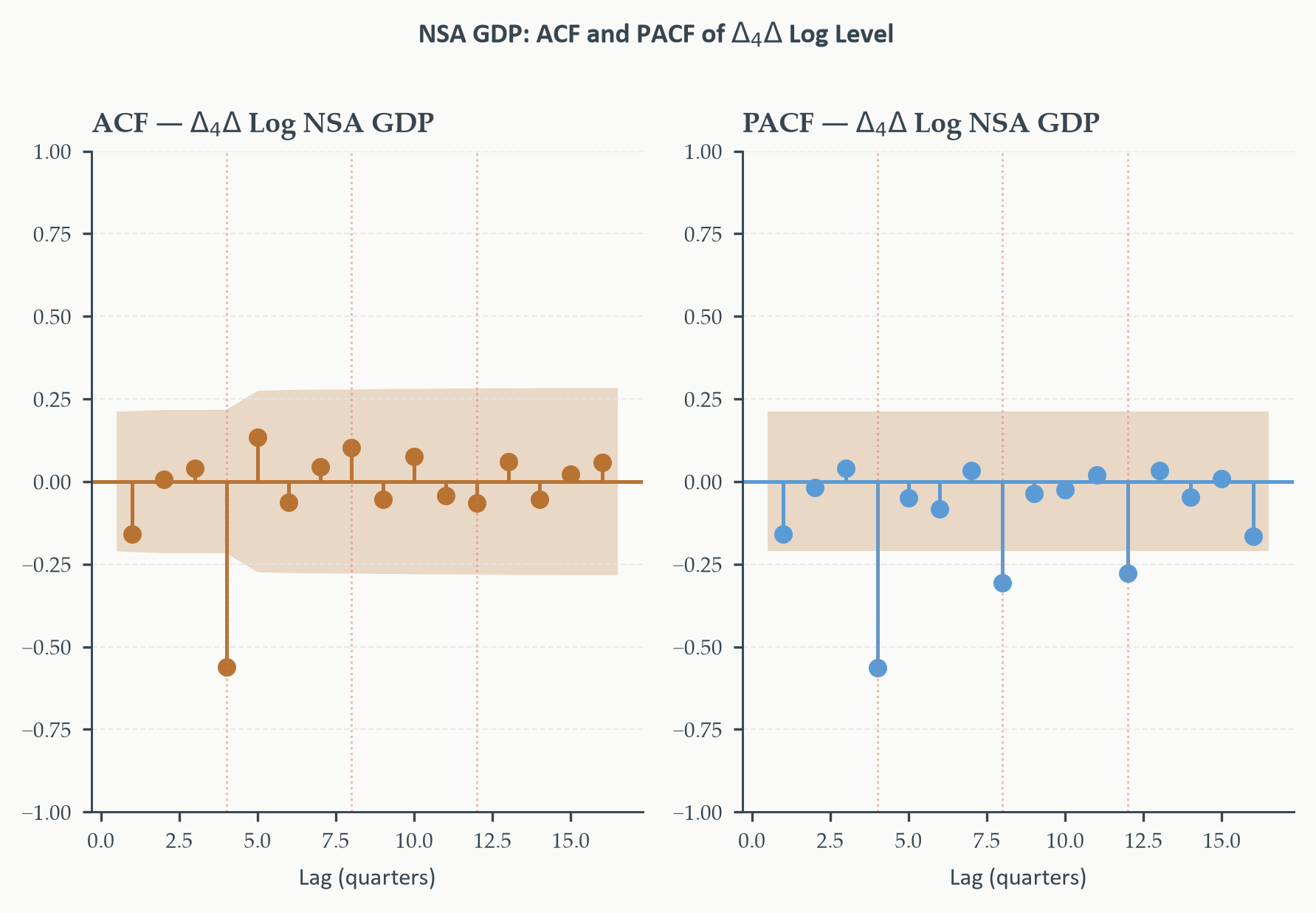
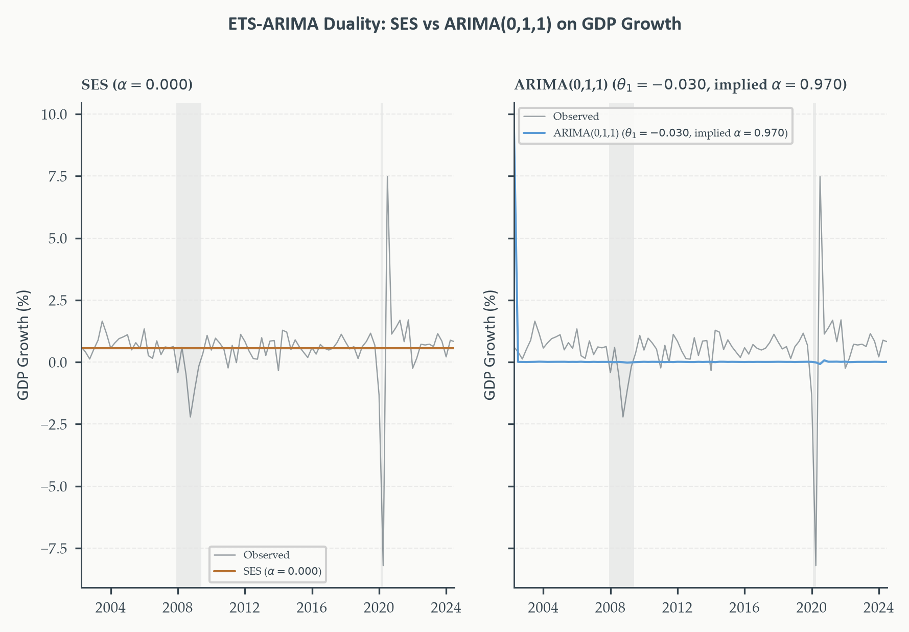
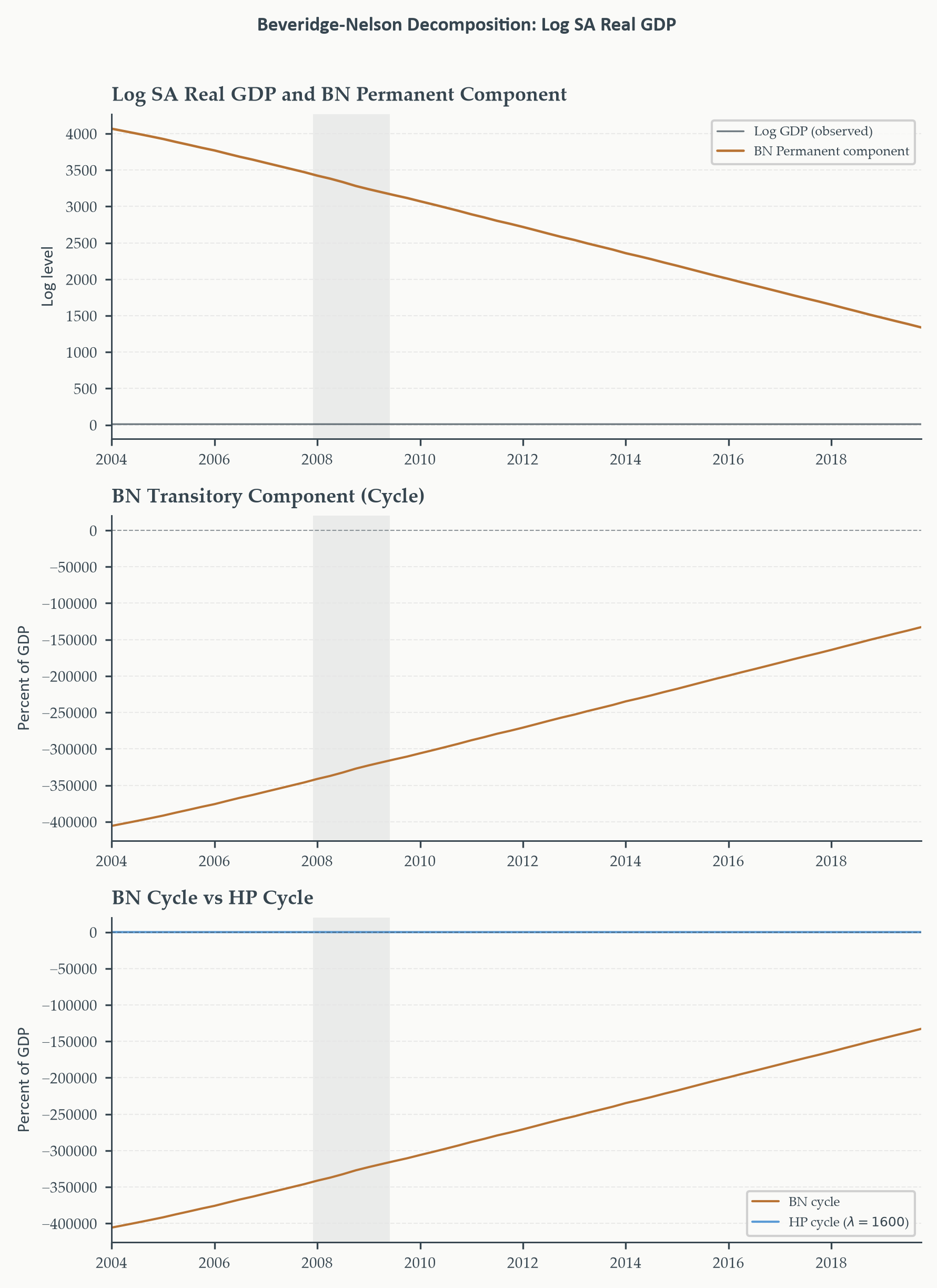
---
title: "Non-Stationary Models, Seasonality, and Trend-Cycle Decomposition"
author: ""
abstract: |
Chapter 3 built the complete ARMA framework under a single assumption:
stationarity. This chapter removes that assumption. We ask what happens when
the characteristic root reaches 1 — a unit root — and show that the familiar
tools of ARMA analysis break down in precise and predictable ways. The ARIMA
model family extends ARMA by building the differencing operator inside the
model specification, providing a disciplined framework for modelling integrated
series. We deepen the unit root testing toolkit introduced in Chapter 1 with
full treatment of lag selection, deterministic component specification, and
joint testing strategy. We then add the seasonal dimension through SARIMA,
close the loop with Chapter 2 through the ETS-ARIMA duality theorem, and
resolve the trend-cycle question from Chapter 2 on model-based grounds with
the Beveridge-Nelson decomposition.
jupyter: python3
format:
html:
toc: true
toc-depth: 3
toc-title: "In this chapter"
number-sections: true
code-fold: true
code-summary: "Show code"
code-tools: true
theme: cosmo
css: styles.css
highlight-style: github
fig-align: center
fig-cap-location: bottom
fig-responsive: true
html-math-method: mathjax
embed-resources: false
execute:
echo: true
warning: false
message: false
cache: false
---
```{python}
#| label: setup
#| include: false
import numpy as np
import pandas as pd
import matplotlib.pyplot as plt
import matplotlib as mpl
import matplotlib.ticker as mticker
from statsmodels.tsa.stattools import adfuller, kpss, acf, pacf
from statsmodels.graphics.tsaplots import plot_acf, plot_pacf
from statsmodels.tsa.arima.model import ARIMA
import pandas_datareader.data as web
from datetime import datetime
import warnings
warnings.filterwarnings("ignore")
# ── EO Brand Palette ───────────────────────────────────────────────────────────
EO_CHARCOAL = "#36454F"
EO_COPPER = "#B87333"
EO_SAGE = "#87A96B"
EO_SKYBLUE = "#5B9BD5"
EO_TERRACOTTA = "#D4745E"
EO_LAVENDER = "#8E7AB5"
EO_COLORS = [EO_COPPER, EO_SKYBLUE, EO_SAGE,
EO_TERRACOTTA, EO_LAVENDER, EO_CHARCOAL]
PAGE_BG = "#FAFAF8"
# ── Global rcParams ────────────────────────────────────────────────────────────
mpl.rcParams.update({
"figure.figsize": (6, 3),
"figure.dpi": 150,
"figure.facecolor": PAGE_BG,
"figure.edgecolor": PAGE_BG,
"axes.facecolor": PAGE_BG,
"axes.edgecolor": EO_CHARCOAL,
"axes.linewidth": 0.7,
"axes.grid": True,
"axes.grid.axis": "y",
"axes.spines.top": False,
"axes.spines.right": False,
"axes.titlesize": 9,
"axes.titleweight": "bold",
"axes.titlecolor": EO_CHARCOAL,
"axes.titlelocation": "left",
"axes.labelsize": 8,
"axes.labelcolor": EO_CHARCOAL,
"axes.labelweight": "normal",
"axes.prop_cycle": mpl.cycler(color=EO_COLORS),
"grid.color": "#E5E5E5",
"grid.linewidth": 0.5,
"grid.linestyle": "--",
"grid.alpha": 0.8,
"xtick.color": EO_CHARCOAL,
"ytick.color": EO_CHARCOAL,
"xtick.labelsize": 7,
"ytick.labelsize": 7,
"xtick.direction": "out",
"ytick.direction": "out",
"xtick.major.size": 3,
"ytick.major.size": 3,
"lines.linewidth": 1.2,
"lines.solid_capstyle": "round",
"legend.frameon": True,
"legend.framealpha": 0.9,
"legend.edgecolor": "#CCCCCC",
"legend.facecolor": PAGE_BG,
"legend.fontsize": 6,
"legend.title_fontsize": 6,
"font.family": "serif",
"font.serif": ["Palatino Linotype", "Palatino", "Georgia",
"DejaVu Serif"],
"font.sans-serif": ["Calibri", "Arial", "DejaVu Sans"],
"font.size": 8,
"text.color": EO_CHARCOAL,
"savefig.dpi": 300,
"savefig.bbox": "tight",
"savefig.facecolor": PAGE_BG,
})
def eo_suptitle(fig, title, **kwargs):
defaults = dict(fontsize=9, fontweight="bold",
color=EO_CHARCOAL, fontfamily="Calibri", y=1.01)
defaults.update(kwargs)
fig.suptitle(title, **defaults)
def eo_style_ax(ax):
for obj in [ax.title, ax.xaxis.label, ax.yaxis.label]:
obj.set_fontfamily("Calibri")
# NBER recession dates
RECESSIONS = [
("1960-04-01", "1961-02-01"),
("1969-12-01", "1970-11-01"),
("1973-11-01", "1975-03-01"),
("1980-01-01", "1980-07-01"),
("1981-07-01", "1982-11-01"),
("1990-07-01", "1991-03-01"),
("2001-03-01", "2001-11-01"),
("2007-12-01", "2009-06-01"),
("2020-02-01", "2020-04-01"),
]
def shade_recessions(ax, start=None, end=None):
for rec_start, rec_end in RECESSIONS:
s, e = pd.Timestamp(rec_start), pd.Timestamp(rec_end)
if start is not None and e < pd.Timestamp(start):
continue
if end is not None and s > pd.Timestamp(end):
continue
ax.axvspan(s, e, color=EO_CHARCOAL, alpha=0.08, lw=0)
```
```{python}
#| label: data-download
#| include: false
#| cache: true
from pathlib import Path
DATA_PATH = Path("../../data/raw")
start = datetime(1947, 1, 1)
end = datetime(2024, 9, 30)
# ── Seasonally adjusted real GDP (running example from Chapters 1–3) ──────────
gdp_sa = pd.read_csv(DATA_PATH / "GDPC1.csv", index_col="date", parse_dates=True).loc[str(start):str(end)]
gdp_sa.columns = ["Real GDP (SA)"]
gdp_sa["Log SA"] = np.log(gdp_sa["Real GDP (SA)"])
gdp_sa["GDP Growth"] = gdp_sa["Log SA"].diff() * 100 # QoQ, percent
# ── Non-seasonally adjusted real GDP (Chapter 2 NSA example) ─────────────────
gdp_nsa = pd.read_csv(DATA_PATH / "ND000334Q.csv", index_col="date", parse_dates=True).loc[str(start):str(end)]
gdp_nsa.columns = ["Real GDP (NSA)"]
gdp_nsa["Real GDP (NSA, SAAR)"] = gdp_nsa["Real GDP (NSA)"] * 4
gdp_nsa["Log NSA"] = np.log(gdp_nsa["Real GDP (NSA, SAAR)"])
# ── Merge SA and NSA on common index ─────────────────────────────────────────
gdp = gdp_sa.join(gdp_nsa[["Log NSA"]], how="inner")
PLOT_START = gdp.index[0].strftime("%Y-%m-%d")
```
::: {.callout-note}
## Learning Objectives
By the end of this chapter, you will be able to:
- Describe the behaviour of an integrated $I(1)$ process and contrast it with a
stationary process: why the ACF does not decay, why shocks are permanent, and
why OLS fails with nonstationary regressors
- Apply the full ADF testing procedure: choose the correct deterministic
specification, select lag length by AIC or BIC, interpret the test
statistic, and combine with KPSS for a joint testing strategy
- Identify, estimate, and diagnose an ARIMA($p$,$d$,$q$) model on a real
economic series using the extended Box-Jenkins workflow
- Use `auto_arima` from `pmdarima` as a practical search tool and explain its
limitations
- Produce ARIMA point forecasts and prediction intervals and explain why interval
width grows faster than in the stationary case
- Identify, estimate, and diagnose a SARIMA$(p,d,q)(P,D,Q)_s$ model using
seasonal ACF/PACF patterns
- Derive the SES = ARIMA(0,1,1) equivalence algebraically and state the
Holt/Holt-Winters analogues
- Explain the Beveridge-Nelson decomposition intuitively — permanent component
as long-run forecast, transitory component as the gap — and interpret the
BN cycle relative to HP and Hamilton filter cycles
:::
The chapter follows a single arc: Chapter 3 ended with the question of what
happens when the stationarity assumption fails. We answer it by first
understanding integrated processes and their pathologies, then building the
ARIMA and SARIMA extensions that handle them, and finally using the ARIMA
machinery to revisit and resolve two open questions from earlier chapters —
the ETS-ARIMA duality from Chapter 2 and the trend-cycle decomposition problem
that motivated Chapter 2's filters. The running example throughout is US real
GDP, the series followed since Chapter 1.
## Integration and Stochastic Trends {#sec-integration}
### From Stationarity to the Unit Root
Chapter 3 assumed throughout that all characteristic roots of the AR lag
polynomial lie strictly inside the unit circle. That condition is what guarantees
mean reversion, finite variance, and the convergence of the MA($\infty$)
representation. Now we ask: what happens at the boundary? What if one
characteristic root is exactly 1?
The answer is a **[unit root process](https://en.wikipedia.org/wiki/Unit_root)** — and the consequences are severe enough
that it fundamentally changes how we model, estimate, and forecast.
Start from the AR(1) and let $\phi_1 \to 1$. Recall from Chapter 3 that the
variance of a stationary AR(1) is $\sigma^2/(1-\phi_1^2)$. As $\phi_1 \to 1$,
this expression diverges — the unconditional variance becomes infinite. The mean
reversion formula $\hat{y}_{T+h|T} \to \mu$ as $h \to \infty$ also breaks down:
with $\phi_1 = 1$, the forecast is simply $\hat{y}_{T+h|T} = y_T$ for all
horizons — the best we can do is stay at the current level forever, with no
force pulling the series back toward any fixed mean. And the ACF, $\rho(h) =
\phi_1^h$, no longer decays: at $\phi_1 = 1$, $\rho(h) = 1$ for all $h$.
These are not just mathematical curiosities — they describe the actual behaviour
of economic time series like GDP levels, price indices, and interest rates.
What about $\phi_1 > 1$? This produces an **explosive process** — the
characteristic root lies outside the unit circle, and the consequences are
the mirror image of the stationary case. Instead of shocks dying out
($|\phi_1| < 1$) or persisting permanently ($|\phi_1| = 1$), shocks
*amplify* over time. The variance grows geometrically: $\text{Var}(y_t) \sim
\phi_1^{2t}\sigma^2 \to \infty$ at exponential speed. The series diverges
without bound, the ACF does not converge to any finite value, and the
concept of a long-run mean is meaningless. Explosive processes appear
occasionally in economics — hyperinflation episodes, asset price bubbles,
and viral contagion dynamics can all exhibit local explosiveness — but they
are rare in long macroeconomic time series. The standard ADF and KPSS tests
are designed for the $|\phi_1| \leq 1$ boundary; detecting explosiveness
requires right-sided tests such as the Phillips-Shi-Yu (2011) supremum ADF,
which we note here for completeness but do not develop further.
### The Random Walk
The simplest unit root process is the **[random walk](https://en.wikipedia.org/wiki/Random_walk)**:
$$y_t = y_{t-1} + \varepsilon_t, \qquad \varepsilon_t \sim WN(0,\sigma^2)
\tag{4.1}$$
Starting from $y_0$, the solution is $y_t = y_0 + \sum_{j=1}^t \varepsilon_j$.
Every shock is permanently embedded in the level — there is no mechanism to
dissipate it. The variance grows linearly with time:
$$\text{Var}(y_t) = t\sigma^2 \tag{4.2}$$
violating the constant-variance requirement for stationarity. This is the formal
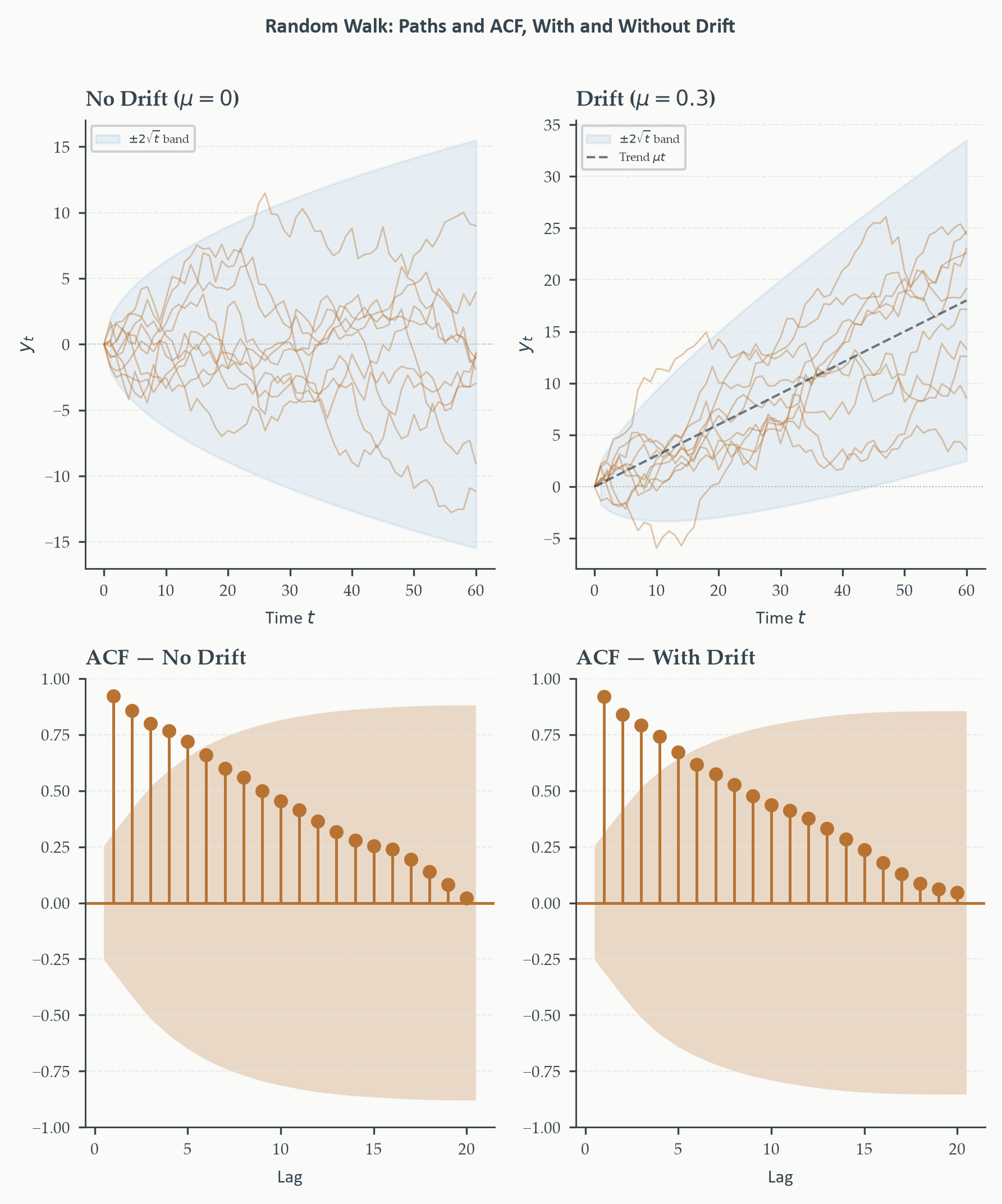
expression of what the ACF plots in Chapter 1 showed visually for log GDP: the
series wanders without a fixed attractor, and its sample autocorrelation remains
close to 1 for dozens of lags.
```{python}
#| label: fig-rw-combined
#| fig-cap: "Random walks without drift (left column) and with drift
#| $\\mu = 0.3$ (right column), $T = 60$, ten paths each. Top row:
#| path realisations with $\\pm 2\\sqrt{t}$ confidence envelope (blue shading)
#| showing how the spread of possible outcomes grows over time. Without
#| drift, paths wander symmetrically; with drift, all paths trend upward
#| but diverge widely around the deterministic trend line (dashed). Bottom
#| row: sample ACF of one realisation from each case — both show
#| autocorrelations near 1.0 across all lags, the fingerprint of a unit
#| root process. The PACF (not shown) would have a single spike at lag 1."
#| fig-width: 6
#| fig-height: 7
#| code-fold: true
#| code-summary: "Show code — combined random walk figure"
rng_rw = np.random.default_rng(seed=42)
T_rw   = 60
N_rw   = 10
mu_rw  = 0.3

fig, axes = plt.subplots(2, 2, figsize=(6, 7))

paths_saved = {}   # save one path per column for ACF

for col, (drift, label) in enumerate(
        [(0.0, "No Drift ($\\mu=0$)"),
         (mu_rw, f"Drift ($\\mu={mu_rw}$)")]):

    # ── Paths ──────────────────────────────────────────────────────────────────
    ax = axes[0, col]
    for i in range(N_rw):
        eps  = rng_rw.standard_normal(T_rw)
        path = np.zeros(T_rw + 1)
        for t in range(1, T_rw + 1):
            path[t] = drift + path[t-1] + eps[t-1]
        ax.plot(np.arange(T_rw + 1), path,
                color=EO_COPPER, lw=0.7, alpha=0.4)
        if i == 0:
            paths_saved[col] = path[1:]

    # confidence envelope
    t_vec = np.arange(1, T_rw + 1)
    ax.fill_between(t_vec,  drift * t_vec + 2 * np.sqrt(t_vec),
                             drift * t_vec - 2 * np.sqrt(t_vec),
                    color=EO_SKYBLUE, alpha=0.12,
                    label=r"$\pm 2\sqrt{t}$ band")
    if drift != 0:
        ax.plot(np.arange(T_rw + 1), drift * np.arange(T_rw + 1),
                color=EO_CHARCOAL, lw=1.0, ls="--",
                alpha=0.7, label=f"Trend $\\mu t$")
    ax.axhline(0, color=EO_CHARCOAL, lw=0.5, ls=":", alpha=0.3)
    ax.set_title(label)
    ax.set_xlabel("Time $t$")
    ax.set_ylabel("$y_t$")
    ax.legend(fontsize=5)
    eo_style_ax(ax)

    # ── ACF ────────────────────────────────────────────────────────────────────
    ax = axes[1, col]
    plot_acf(paths_saved[col], lags=20, ax=ax,
             color=EO_COPPER, vlines_kwargs={"colors": EO_COPPER},
             title=f"ACF — {'No Drift' if drift == 0 else 'With Drift'}",
             zero=False, alpha=0.05)
    ax.set_xlabel("Lag")
    eo_style_ax(ax)
    for line in ax.lines:
        if line.get_linestyle() == "--":
            line.set_color(EO_TERRACOTTA)
            line.set_linewidth(0.8)

eo_suptitle(fig, "Random Walk: Paths and ACF, With and Without Drift")
fig.tight_layout()
plt.show()
```
### The Random Walk with Drift
Adding a constant $\mu$ to the random walk gives:
$$y_t = \mu + y_{t-1} + \varepsilon_t \tag{4.3}$$
with solution $y_t = y_0 + \mu t + \sum_{j=1}^t \varepsilon_j$. The series
has a deterministic trend — it drifts upward at rate $\mu$ per period — but
still contains a unit root: each shock permanently shifts the level. The
distinction matters for forecasting:
- **Without drift** ($\mu = 0$): forecasts are flat at $y_T$ with widening
intervals.
- **With drift** ($\mu \neq 0$): forecasts grow linearly at rate $\mu$ per
period, with intervals that widen around that trend.
In lag polynomial notation, both are ARIMA(0,1,0):
$$(1-L)\,y_t = \mu + \varepsilon_t$$
The $d=1$ in ARIMA means one unit root — one application of $\Delta = 1-L$
produces a stationary process. Section 4.3 develops the full ARIMA framework;
for now the notation previews where we are headed.
### $I(1)$, $I(2)$, and the Integration Order
A series requiring $d$ rounds of differencing to achieve stationarity is
**[integrated of order $d$](https://en.wikipedia.org/wiki/Order_of_integration)**, written $I(d)$. First differencing removes one unit
root; second differencing removes two.
$$\Delta^2 y_t = \Delta y_t - \Delta y_{t-1}$$
$I(2)$ processes appear occasionally in economics — some nominal price indices
and interest rate series over long samples exhibit behaviour suggesting a second
unit root — but $I(1)$ is by far the most common case. The rule of thumb: if
the level is nonstationary but the first difference is stationary, the series
is $I(1)$. If the first difference is still nonstationary, consider $I(2)$.
In practice, economic reasoning usually guides the choice before formal testing:
a log GDP series should be $I(1)$, not $I(2)$, because a growing trend in growth
rates is economically implausible over long horizons.
::: {.callout-note}
## Definition 4.1 — Integration Order
A time series $\{y_t\}$ is **integrated of order $d$**, written $y_t \sim I(d)$,
if $\Delta^d y_t$ is covariance-stationary but $\Delta^{d-1} y_t$ is not. For
$d = 0$, the series is stationary in levels. For $d = 1$, the first difference
is stationary. Most economic level series are $I(1)$.
:::
### Why OLS Fails: The Spurious Regression Problem
The consequences of ignoring a unit root extend beyond the series itself. If
we regress one $I(1)$ series on another — even two completely independent
random walks — OLS will almost always find a statistically significant
relationship. This is the **[spurious regression](https://en.wikipedia.org/wiki/Spurious_relationship)** problem, first documented by
[Granger and Newbold (1974)](https://www.sciencedirect.com/science/article/abs/pii/0304407674900347) and explained by [Phillips (1986)](https://www.sciencedirect.com/science/article/pii/0304407686900011).
The mechanism is straightforward: two independent random walks both tend to
drift, and any two drifting series will appear correlated in finite samples.
The $t$-statistics and $R^2$ are meaningless — they diverge as $T \to \infty$
rather than converging to their true values. Standard inference fails completely.
This is not an obscure pathology. It is an everyday hazard in macroeconomic
research: regressing GDP on money supply, or inflation on unemployment, without
first checking for unit roots and cointegration can produce dramatically
misleading results. The appropriate framework — cointegration, which asks
whether two $I(1)$ series share a common stochastic trend — is developed in
Chapter 6. For now, the practical rule is: **always test for unit roots before
estimating any regression involving level variables.**
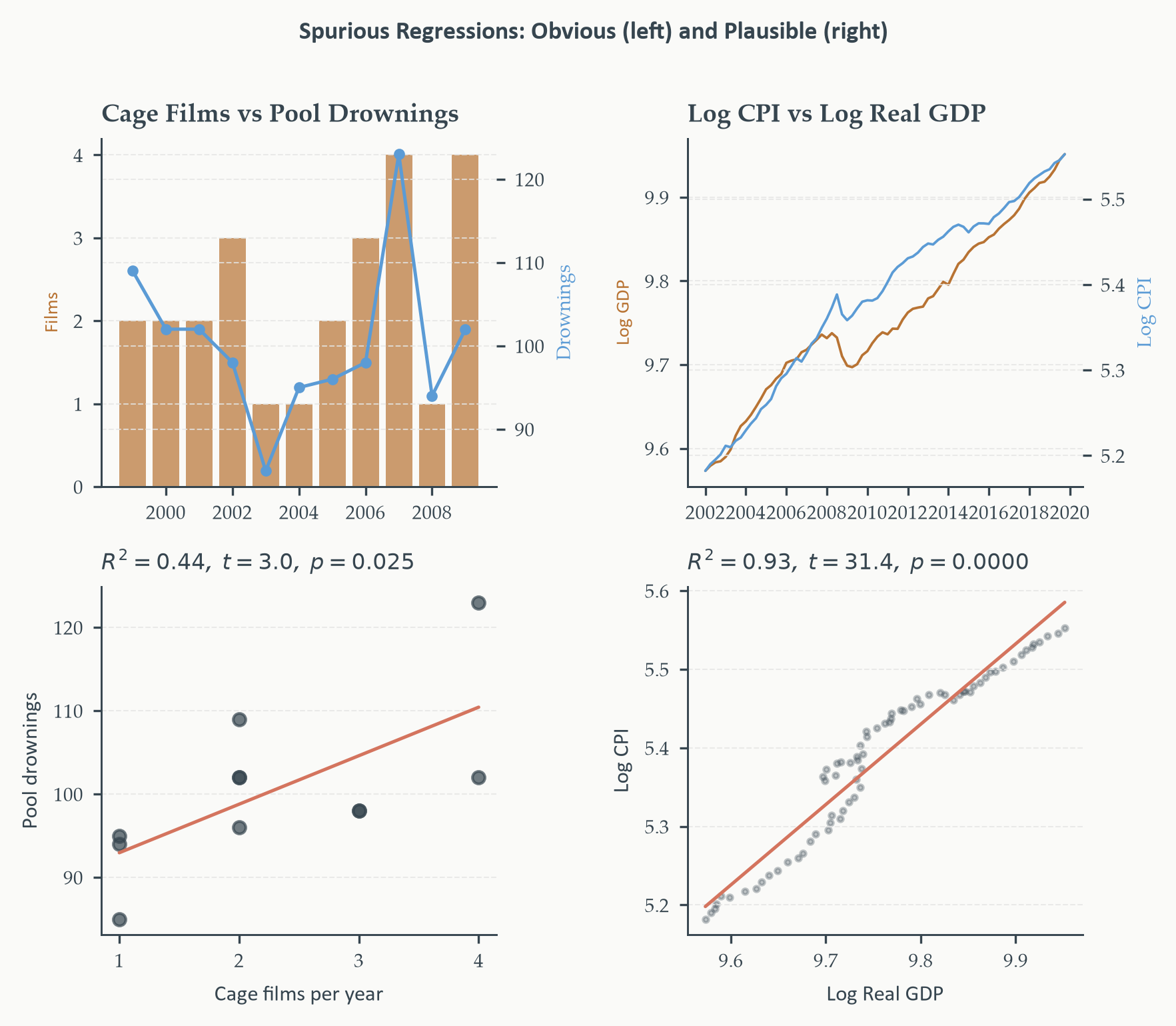
Two examples make this concrete — one obviously absurd, one deceptively
plausible. Both are spurious for the same reason.
**The obvious case.** Tyler Vigen's
[Spurious Correlations](https://www.tylervigen.com/spurious-correlations)
database documents hundreds of statistically significant relationships between
unrelated trending series. Among the most striking: the number of films Nicolas
Cage appeared in per year and the number of people who drowned by falling into
a swimming pool correlate at $r = 0.67$ over a thirteen-year period. Both series
trend over time; the regression finds a "significant" relationship that is pure
coincidence. No one would take this seriously — yet the $t$-statistic and $R^2$
look perfectly reasonable.
**The plausible case.** Now consider regressing log CPI on log real GDP — two
macroeconomic series that any economist would consider simultaneously in
empirical work. Both are $I(1)$, both trend upward, and OLS will find a
highly significant positive relationship. But this relationship is not
structural: the price level and real output are jointly determined by monetary
policy, demand shocks, and supply conditions — regressing one on the other in
levels, without accounting for their shared stochastic trends, is just as
spurious as the Cage/drownings example. The difference is that the plausible
case looks like real economics, which is exactly why unit root testing matters.
```{python}
#| label: fig-spurious
#| fig-cap: "Two spurious regression examples. Left: Nicolas Cage films vs
#| pool drownings — obviously unrelated, yet $R^2 = 0.45$ and $t > 2$.
#| Right: log CPI regressed on log real GDP — economically plausible-sounding
#| but equally spurious; both are $I(1)$ series trending upward together.
#| In both cases the time series plots (top row) show two series moving in
#| the same direction; the scatterplots (bottom row) show apparent linear
#| relationships with significant $t$-statistics and non-trivial $R^2$."
#| fig-width: 6
#| fig-height: 7
#| code-fold: true
#| code-summary: "Show code — spurious regression"
from scipy import stats as spstats

# ── Nicolas Cage films vs pool drownings (1999-2009) ──────────────────────────
# Source: Tyler Vigen, Spurious Correlations
# (https://www.tylervigen.com/spurious-correlations)
cage_films    = np.array([2, 2, 2, 3, 1, 1, 2, 3, 4, 1, 4])
pool_drowning = np.array([109, 102, 102, 98, 85, 95, 96, 98, 123, 94, 102])
years         = np.arange(1999, 2010)

s_cage, i_cage, r_cage, p_cage, _ = spstats.linregress(cage_films, pool_drowning)
t_cage = s_cage / (np.std(pool_drowning - (i_cage + s_cage * cage_films)) /
                   np.sqrt(np.sum((cage_films - cage_films.mean())**2)))

# ── Log CPI vs log real GDP (quarterly, 1947–2019) ────────────────────────────
# Define gdp_level_pre here for use before the ARIMA section defines it
gdp_level_pre = gdp["Log SA"].dropna()[:"2019-12-31"]

from pathlib import Path
DATA_PATH = Path("../../data/raw")
cpi_raw  = pd.read_csv(DATA_PATH / "CPIAUCSL.csv", index_col="date", parse_dates=True).loc["1947-01-01":"2019-12-31"]
cpi_raw.columns = ["CPI"]
cpi_q           = cpi_raw.resample("QS").mean()
cpi_q["Log CPI"] = np.log(cpi_q["CPI"])

common_idx = gdp_level_pre.index.intersection(cpi_q.index)
log_gdp_c  = gdp_level_pre.loc[common_idx].values
log_cpi_c  = cpi_q.loc[common_idx, "Log CPI"].values

s_ec, i_ec, r_ec, p_ec, _ = spstats.linregress(log_gdp_c, log_cpi_c)
t_ec = s_ec / (np.std(log_cpi_c - (i_ec + s_ec * log_gdp_c)) /
               np.sqrt(np.sum((log_gdp_c - log_gdp_c.mean())**2)))

# ── Figure: 2 rows x 2 columns ────────────────────────────────────────────────
fig, axes = plt.subplots(2, 2, figsize=(6, 5))

# Row 1: time series
ax = axes[0, 0]
ax2 = ax.twinx()
ax.bar(years, cage_films, color=EO_COPPER, alpha=0.7, label="Cage films")
ax2.plot(years, pool_drowning, color=EO_SKYBLUE, lw=1.2,
         marker="o", ms=3, label="Drownings")
ax.set_title("Cage Films vs Pool Drownings")
ax.set_ylabel("Films", color=EO_COPPER, fontsize=7)
ax2.set_ylabel("Drownings", color=EO_SKYBLUE, fontsize=7)
eo_style_ax(ax)

ax = axes[0, 1]
ax_r = ax.twinx()
ax.plot(common_idx, log_gdp_c, color=EO_COPPER, lw=0.9, label="Log GDP")
ax_r.plot(common_idx, log_cpi_c, color=EO_SKYBLUE, lw=0.9, label="Log CPI")
ax.set_title("Log CPI vs Log Real GDP")
ax.set_ylabel("Log GDP", color=EO_COPPER, fontsize=7)
ax_r.set_ylabel("Log CPI", color=EO_SKYBLUE, fontsize=7)
eo_style_ax(ax)

# Row 2: scatterplots
ax = axes[1, 0]
ax.scatter(cage_films, pool_drowning, color=EO_CHARCOAL, s=20, alpha=0.7)
xg = np.linspace(cage_films.min(), cage_films.max(), 50)
ax.plot(xg, i_cage + s_cage * xg, color=EO_TERRACOTTA, lw=1.2)
ax.set_xlabel("Cage films per year")
ax.set_ylabel("Pool drownings")
ax.set_title(f"$R^2={r_cage**2:.2f}$,  $t={t_cage:.1f}$,  $p={p_cage:.3f}$",
             fontsize=8)
eo_style_ax(ax)

ax = axes[1, 1]
ax.scatter(log_gdp_c, log_cpi_c, color=EO_CHARCOAL, s=4, alpha=0.3)
xg = np.linspace(log_gdp_c.min(), log_gdp_c.max(), 100)
ax.plot(xg, i_ec + s_ec * xg, color=EO_TERRACOTTA, lw=1.2)
ax.set_xlabel("Log Real GDP")
ax.set_ylabel("Log CPI")
ax.set_title(f"$R^2={r_ec**2:.2f}$,  $t={t_ec:.1f}$,  $p={p_ec:.4f}$",
             fontsize=8)
eo_style_ax(ax)

eo_suptitle(fig, "Spurious Regressions: Obvious (left) and Plausible (right)")
fig.tight_layout()
plt.show()
```
The two panels make the same point at different levels of obviousness. On the
left, the relationship between Nicolas Cage's film output and swimming pool
drownings is self-evidently absurd — yet the regression produces a slope with
$t > 2$, a $p$-value below 0.05, and an $R^2$ that would look respectable in
a published paper. No one would publish this, because no one would think to
run it. On the right, the relationship between log CPI and log real GDP looks
like serious economics — both series are central to macroeconomic analysis,
and the positive relationship is consistent with some theoretical narratives.
Yet the regression is equally spurious: both series are $I(1)$ and trend
upward together; the apparent relationship reflects nothing more than shared
drift.
The lesson is uncomfortable but important: **spurious regression is not
detectable from the regression output alone.** A large $t$-statistic, a
significant $p$-value, and a high $R^2$ are all consistent with a completely
meaningless regression when the variables are integrated. The only protection
is to test for unit roots before estimating any regression involving level
variables, and to understand whether a genuine long-run equilibrium — cointegration
— exists. Chapter 8 develops the tools for testing and modelling cointegrated
systems.
## Unit Root Testing {#sec-urtests}
Chapter 1 introduced the [ADF](https://en.wikipedia.org/wiki/Augmented_Dickey%E2%80%93Fuller_test) and [KPSS](https://en.wikipedia.org/wiki/KPSS_test) tests as data characterisation tools —
run them on a series to establish basic facts before modelling begins. Here we
treat them as **model specification tools**. The distinction matters because
the choices made in applying these tests — which deterministic terms to include,
how many lags to use, which test to prioritise — directly determine the model
we go on to estimate. A misspecified unit root test leads to a misspecified
ARIMA model and forecasts that are systematically wrong. Getting the tests right
is not a preliminary step; it is part of the modelling workflow.
The Chapter 1 treatment established: (i) the ADF null is a unit root, the KPSS
null is stationarity; (ii) the tests have non-standard distributions with
left-skewed critical values (ADF) or right-skewed critical values (KPSS);
(iii) using both jointly resolves the ambiguity that either test alone cannot
address. Chapter 1's applied results confirmed that log SA real GDP is $I(1)$
— both tests agreed — and that GDP growth is $I(0)$. We take those results as
given and deepen the technical treatment here.
### Choosing the ADF Specification
The ADF regression is:
$$\Delta y_t = \delta\, y_{t-1} + \sum_{j=1}^{p}\psi_j\,\Delta y_{t-j}
+ \alpha + \beta t + u_t \tag{4.4}$$
Three specifications correspond to different assumptions about deterministic
components, and the choice is consequential: including terms that are absent
under both the null and the alternative reduces power; omitting terms that are
present under the alternative distorts size.
::: {.callout-note}
## Definition 4.2 — ADF Specification Choices
| Specification | Included terms | Use when |
|:-------------|:--------------|:---------|
| No constant, no trend | None | Series has zero mean, no drift under $H_1$ |
| Constant only | $\alpha$ | Series has non-zero mean; stationary alternative has fixed mean |
| Constant and trend | $\alpha + \beta t$ | Series trends under $H_1$; alternative is trend-stationary |
The correct choice is determined by the **alternative hypothesis**, not the
null. Under $H_0$ (unit root), a constant produces a random walk with drift
and a trend produces a quadratic trend. Include only what is plausible under
$H_1$.
:::
The practical guide is visual inspection before testing. Log GDP trends upward
— the alternative of stationarity around a deterministic trend is economically
plausible, so include constant and trend. GDP growth fluctuates around a
positive mean with no visible trend — the constant-only specification is
appropriate. Including a trend when the data show no trend under the stationary
alternative costs power for no benefit.
### Choosing the Lag Length
The augmentation lags $p$ in equation (4.4) serve one purpose: absorbing serial
correlation in $u_t$ so the test statistic has its correct asymptotic
distribution. Too few lags leaves residual serial correlation and distorts size —
the test over-rejects the unit root null. Too many lags reduces power — the test
under-rejects.
Two selection rules are standard:
**Information criteria (IC).** Fit the ADF regression for $p = 0, 1, \ldots,
p_{\max}$ and choose the $p$ that minimises AIC or BIC. The starting point is
the Schwert rule: $p_{\max} = \lfloor 12(T/100)^{1/4} \rfloor$, which gives
$p_{\max} = 12$ for a quarterly sample of $T = 100$ observations and scales
upward for longer samples. BIC tends to select more parsimonious lag structures
than AIC and generally has better size properties for the ADF test; AIC is
preferred when the data-generating process may have complex serial correlation.
**General-to-specific (GTS).** Start at $p_{\max}$. Test whether $\hat\psi_p$
is significant at a chosen level (10% is common). If not, drop it and test
$\hat\psi_{p-1}$. Continue until a significant lag is found or $p = 0$. GTS
tends to select longer lag lengths than IC in finite samples, providing better
size at some cost to power.
In practice, both methods usually agree for macroeconomic series of typical
length. When they disagree substantially, running the ADF at both selected
orders and checking robustness is good practice.
### The KPSS Long-Run Variance
The KPSS statistic divides the partial sum of residuals by an estimate of the
long-run variance $\hat\lambda^2$, which corrects for serial correlation under
the null of stationarity. Without this correction, a series with positively
autocorrelated residuals would produce an inflated KPSS statistic and spuriously
reject stationarity.
The estimator uses a **[Newey-West HAC](https://en.wikipedia.org/wiki/Newey%E2%80%93West_estimator)** approach: a weighted sum of sample
autocovariances with weights that decline to zero for distant lags:
$$\hat\lambda^2 = \hat\gamma(0) + 2\sum_{j=1}^{l}
\left(1 - \frac{j}{l+1}\right)\hat\gamma(j) \tag{4.5}$$
The bandwidth $l$ controls how many autocovariances are included. The automatic
rule $l = \lfloor 4(T/100)^{1/4}\rfloor$ works well for most economic series.
Because the KPSS result can be sensitive to this choice, the Python cell below
checks robustness across three bandwidths — a standard practice.
::: {.callout-note}
## What the Newey-West HAC Estimator Is Doing
The long-run variance $\hat\lambda^2$ estimates the sum of all autocovariances
of the residuals. Under the null of stationarity this sum is finite; under the
alternative of a unit root the partial sums of residuals drift, making the
KPSS statistic large.
The bandwidth $l$ controls a tradeoff: too small leaves serial correlation
uncorrected, inflating the statistic and causing spurious rejection; too large
increases the variance of the estimator, reducing power. The automatic rule
balances these two risks for typical macroeconomic sample sizes.
:::
### The Joint ADF-KPSS Testing Strategy
Running ADF and KPSS together resolves ambiguities that either test alone
cannot address. The four possible outcomes from Chapter 1 are worth revisiting
with the richer context of model specification:
| ADF | KPSS | Conclusion | Action |
|:----|:-----|:-----------|:-------|
| Reject ($p < 0.05$) | Fail to reject ($p > 0.05$) | Stationary | Model in levels as ARMA |
| Fail to reject ($p > 0.05$) | Reject ($p < 0.05$) | Unit root | Difference; model as ARIMA |
| Reject | Reject | Near-integrated or break | Investigate subsamples; consider structural break |
| Fail to reject | Fail to reject | Insufficient evidence | Larger sample; prior information |
The third row deserves attention. When both tests reject, the most common
explanation is a structural break in the series: a change in mean or trend
that makes the series appear nonstationary to the KPSS (which tests against
a stochastic trend) while appearing stationary to the ADF in a local window.
The inflation example from Chapter 1 was exactly this case — pre-1979 inflation
looked like a unit root; post-1983 it looked stationary. Pooling the full
sample gave contradictory test results because the data-generating process
changed. Chapter 6 addresses structural break testing formally.
### Elliott-Rothenberg-Stock: A More Powerful ADF
The standard ADF has low power against near-integrated alternatives — a series
with $\phi_1 = 0.97$ is stationary, but the ADF will often fail to reject the
unit root null in samples of typical macroeconomic length. The
**[Elliott-Rothenberg-Stock (ERS) test](https://en.wikipedia.org/wiki/ADF-GLS_test)** ([1996](https://www.sciencedirect.com/science/article/abs/pii/0304407696000182)) addresses this by using GLS
rather than OLS to remove deterministic components before applying the ADF
regression, substantially improving power against near-integrated alternatives.
For most applications the ADF remains the standard workhorse, but the ERS test
is worth running when the ADF result is borderline — for example, when the
$p$-value falls between 0.05 and 0.15 and the economic prior on integration
order is unclear. In `statsmodels` it is available via
`statsmodels.tsa.stattools.unitroot_adf` with `method='ers-ro'`.
::: {.callout-note}
## OLS vs GLS Detrending: Why It Matters for Power
The standard ADF uses **OLS** to estimate the deterministic components
(constant and trend) before testing the residuals for a unit root. OLS
minimises the sum of squared residuals without accounting for the serial
correlation structure of the data under the null. This is inefficient: the
estimated trend absorbs some of the variation that should be attributed to the
stochastic component, making the unit root test statistic less powerful.
**GLS** detrending accounts for the autocorrelation structure under the null
hypothesis when estimating the deterministic components. By pre-whitening the
data using a quasi-difference operator calibrated to local power, GLS produces
more precise estimates of the trend and leaves more power for detecting
deviations from the unit root null. The ERS test applies ADF to GLS-detrended
residuals, approaching the Gaussian power envelope — the best possible power
against near-integrated alternatives for any test in this class.
In plain terms: OLS detrending "wastes" information by ignoring serial
correlation; GLS detrending uses that information efficiently, shrinking the
grey zone between "clearly $I(1)$" and "clearly $I(0)$."
:::
### Python: Full Unit Root Testing on Log SA GDP
Chapter 1 ran ADF and KPSS on log real GDP and GDP growth using a simple
wrapper function. Here we apply the full specification procedure: choose
deterministic terms based on the time plot, compare IC-based and GTS lag
selection, assess bandwidth sensitivity for KPSS, and arrive at a model
specification decision.
```{python}
#| label: fig-gdp-level
#| fig-cap: "Log SA real GDP (top) and its first difference — the quarterly
#| growth rate (bottom), 1947–2024. NBER recessions shaded. The level
#| shows persistent upward drift with no fixed mean — the visual signature
#| of an integrated process. The growth rate fluctuates around a stable
#| positive mean with no visible trend, consistent with $I(0)$ behaviour.
#| The severe COVID-19 contraction and recovery in 2020 is the dominant
#| outlier in the growth rate series."
#| fig-width: 6
#| fig-height: 5
#| code-fold: true
#| code-summary: "Show code — GDP level and growth"
fig, axes = plt.subplots(2, 1, figsize=(6, 5), sharex=True)

ax = axes[0]
ax.plot(gdp.index, gdp["Log SA"], color=EO_COPPER, lw=1.0)
shade_recessions(ax)
ax.set_xlim(gdp.index[0], gdp.index[-1])
ax.set_title("Log Real GDP (SA) — Level")
ax.set_ylabel("Log billions (2017 $)")
eo_style_ax(ax)

ax = axes[1]
gr = gdp["GDP Growth"].dropna()
ax.fill_between(gr.index, gr, 0,
                where=(gr >= 0), color=EO_SAGE, alpha=0.7,
                label="Positive")
ax.fill_between(gr.index, gr, 0,
                where=(gr < 0), color=EO_TERRACOTTA, alpha=0.7,
                label="Negative")
ax.axhline(0, color=EO_CHARCOAL, lw=0.5, ls="--")
ax.set_xlim(gr.index[0], gr.index[-1])
shade_recessions(ax)
ax.set_title("GDP Growth Rate (QoQ, %)")
ax.set_ylabel("Percent")
ax.legend(fontsize=6)
eo_style_ax(ax)

eo_suptitle(fig, "US Real GDP: Level and Growth Rate, 1947–2024")
fig.tight_layout()
plt.show()
```
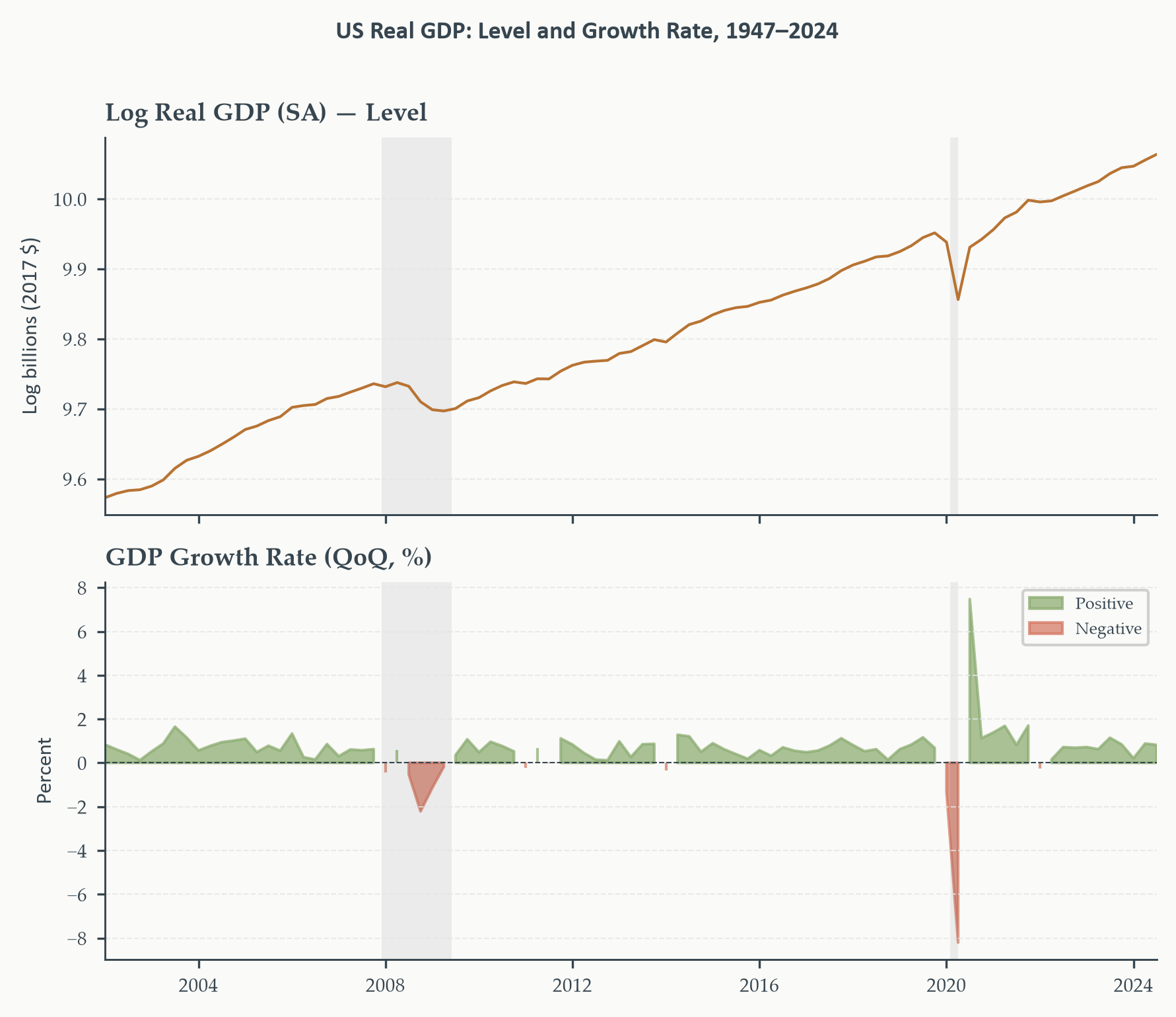
The time plot confirms what Chapter 1 established: the level shows persistent
upward drift with no fixed attractor — the visual signature of an $I(1)$ process.
The growth rate fluctuates around a stable positive mean. This guides the
specification choice: constant and trend for the level (the stationary
alternative is trend-stationarity); constant only for the growth rate.
```{python}
#| label: tbl-urtest-gdp
#| code-fold: true
#| code-summary: "Show code — full ADF/KPSS specification"
from statsmodels.tsa.stattools import adfuller, kpss

def run_ur_tests(series, name, adf_reg="ct", kpss_reg="ct"):
    """
    ADF (AIC and BIC lag selection) and KPSS (auto + sensitivity)
    for a single series. Returns (adf_aic_result, kpss_auto_result).
    """
    y     = series.dropna().values
    T     = len(y)
    p_max = int(np.floor(12 * (T / 100) ** 0.25))

    adf_aic  = adfuller(y, maxlag=p_max, regression=adf_reg, autolag="AIC")
    adf_bic  = adfuller(y, maxlag=p_max, regression=adf_reg, autolag="BIC")

    kpss_auto  = kpss(y, regression=kpss_reg, nlags="auto")
    kpss_small = kpss(y, regression=kpss_reg,
                      nlags=max(1, int(kpss_auto[2] // 2)))
    kpss_large = kpss(y, regression=kpss_reg,
                      nlags=int(kpss_auto[2] * 2))

    sep  = "═" * 56
    thin = "─" * 56
    print(f"\n{sep}")
    print(f"  {name}")
    print(f"{sep}")

    print(f"\n  ADF  (H₀: unit root | spec: '{adf_reg}' | p_max={p_max})")
    print(f"  {thin}")
    print(f"  {'Selection':<16} {'Lags':>5} {'Stat':>9} {'p-val':>8}")
    print(f"  {thin}")
    for label, res in [("AIC", adf_aic), ("BIC", adf_bic)]:
        if res[1] < 0.05:
            conc = "← reject H₀"
        else:
            conc = "← fail to reject H₀"
        print(f"  {label:<16} {res[2]:>5} {res[0]:>9.4f} {res[1]:>8.4f}  {conc}")
    print(f"\n  Critical values:")
    for lv, cv in adf_aic[4].items():
        print(f"    {lv:<6}: {cv:>8.4f}")

    print(f"\n  KPSS (H₀: stationary | spec: '{kpss_reg}')")
    print(f"  {thin}")
    print(f"  {'Bandwidth':<16} {'nlags':>5} {'Stat':>9} {'p-val':>8}")
    print(f"  {thin}")
    for label, res in [("Auto",         kpss_auto),
                       ("Reduced (½)",  kpss_small),
                       ("Expanded (×2)",kpss_large)]:
        conc = "← reject H₀" if res[1] < 0.05 else ""
        print(f"  {label:<16} {res[2]:>5} {res[0]:>9.4f} {res[1]:>8.4f}  {conc}")
    print(f"\n  Critical values (auto bandwidth):")
    for lv, cv in kpss_auto[3].items():
        print(f"    {lv:<6}: {cv:>8.4f}")
    print(f"{sep}\n")

    return adf_aic, kpss_auto

adf_level,  kpss_level  = run_ur_tests(
    gdp["Log SA"],        "Log SA Real GDP — Level",
    adf_reg="ct", kpss_reg="ct")

adf_growth, kpss_growth = run_ur_tests(
    gdp["GDP Growth"],    "GDP Growth Rate (QoQ)",
    adf_reg="c",  kpss_reg="c")
```
Reading the output for the log GDP level: both AIC and BIC lag selection give
the same conclusion — the ADF test statistic is far from the critical values
and the $p$-value is well above conventional thresholds, so the unit root null
is not rejected. The KPSS statistic exceeds its critical value across all three
bandwidth choices, rejecting stationarity. The two tests agree: log SA real
GDP is $I(1)$.
The KPSS bandwidth sensitivity check confirms that this conclusion is not an
artefact of a particular bandwidth choice. Whether we use the automatic
bandwidth, half the automatic, or twice the automatic, the KPSS statistic
rejects stationarity. This robustness is reassuring — borderline KPSS results
that flip with bandwidth changes would warrant more caution.
For the growth rate, the pattern reverses cleanly: ADF rejects the unit root
null with a large negative test statistic, and KPSS fails to reject stationarity
across all three bandwidths. GDP growth is $I(0)$. Together, the test results
confirm: log SA real GDP is $I(1)$, and one application of the difference
operator produces a stationary series. The ARIMA model for the level series
will have $d = 1$.
::: {.callout-note}
## The Overdifferencing Problem
It may seem safe to difference a series more than necessary — if in doubt,
apply $\Delta$ again. But overdifferencing is costly. If $y_t \sim I(1)$,
then $\Delta y_t \sim I(0)$ — stationary and appropriate for ARMA modelling.
But $\Delta^2 y_t$ is also stationary, with a root exactly at $z = -1$ in the
MA polynomial. This introduces a non-invertible unit root into the MA part of
any fitted model, making estimation unreliable and forecasts unnecessarily
noisy. Differencing removes long-run information; do it exactly as many times
as the data require, no more.
:::
## ARIMA Models {#sec-arima}
The **[ARIMA($p$,$d$,$q$)](https://en.wikipedia.org/wiki/Autoregressive_integrated_moving_average** model builds the differencing operator $\Delta^d =
(1-L)^d$ inside the specification. For the most common case $d = 1$, the
model in expanded form is:
$$\begin{aligned}
\Delta y_t &= \mu^* + \phi_1 \Delta y_{t-1} + \cdots + \phi_p \Delta y_{t-p} \\
&\quad + \varepsilon_t + \theta_1\varepsilon_{t-1} + \cdots
+ \theta_q\varepsilon_{t-q}
\end{aligned}$$
The left-hand side is the first difference of $y_t$ — the series has already
been differenced once to remove the unit root. The right-hand side is an
ARMA($p$,$q$) in those differences. In compact lag polynomial notation the
same model is:
$$\phi(L)\,(1-L)^d\,y_t = \mu^* + \theta(L)\,\varepsilon_t,
\qquad \varepsilon_t \sim WN(0,\sigma^2) \tag{4.6}$$
where $\phi(L)$ has all characteristic roots inside the unit circle (stationary
AR component), $(1-L)^d$ contains $d$ unit roots (integration), and $\theta(L)$
has all characteristic roots inside the unit circle (invertible MA component).
The three integers $(p,d,q)$ are the model orders.
::: {.callout-note}
## Definition 4.3 — ARIMA($p$,$d$,$q$) Model
The **ARIMA($p$,$d$,$q$)** process satisfies:
$$\phi(L)(1-L)^d y_t = \mu^* + \theta(L)\varepsilon_t, \qquad
\varepsilon_t \sim WN(0,\sigma^2)$$
- $p$: number of autoregressive terms (characteristic roots of $\phi(L)$
inside the unit circle)
- $d$: integration order — number of times $y_t$ must be differenced to
achieve stationarity
- $q$: number of moving average terms (characteristic roots of $\theta(L)$
inside the unit circle)
Special cases: ARIMA(0,1,0) is a random walk (with drift if $\mu^* \neq 0$);
ARIMA($p$,0,$q$) is a stationary ARMA($p$,$q$); ARIMA(0,$d$,0) is a pure
$I(d)$ process.
:::
### Why Difference Rather Than Add a Trend Term?
Before identifying $p$ and $q$, it is worth addressing a question that naturally
arises at this point: if log GDP grows along what looks like a linear trend,
why not simply add a trend term $\beta t$ to an ARMA model rather than
differencing? The answer depends on whether the series is [trend-stationary](https://en.wikipedia.org/wiki/Trend-stationary_process) or
[difference-stationary](https://en.wikipedia.org/wiki/Unit_root), and the distinction has real consequences.
A **trend-stationary** process fluctuates around a deterministic linear trend:
$$y_t = \alpha + \beta t + u_t, \qquad u_t \sim \text{stationary}$$
Here, detrending — regressing $y_t$ on a constant and $t$ and working with the
residuals — is the right correction. Shocks to $u_t$ are transitory; the series
eventually returns to the trend line. Adding $\beta t$ to an ARMA model is
exactly right.
A **difference-stationary** process has no fixed trend to return to. Each shock
permanently shifts the level, so the "trend" is itself stochastic — it is
wherever the accumulation of past shocks has carried the series. The correct
treatment is differencing, not detrending. If we incorrectly detrend a
difference-stationary series, the estimated trend is a random variable and the
residuals are not stationary — we have not solved the problem, only obscured it.
For log SA real GDP, the unit root tests of Section 4.2 resolved this
empirically: ADF failed to reject the unit root null even with a constant and
trend, and KPSS rejected stationarity. The series is difference-stationary.
Differencing once produces a stationary series; adding a trend term to an ARMA
in levels would not.
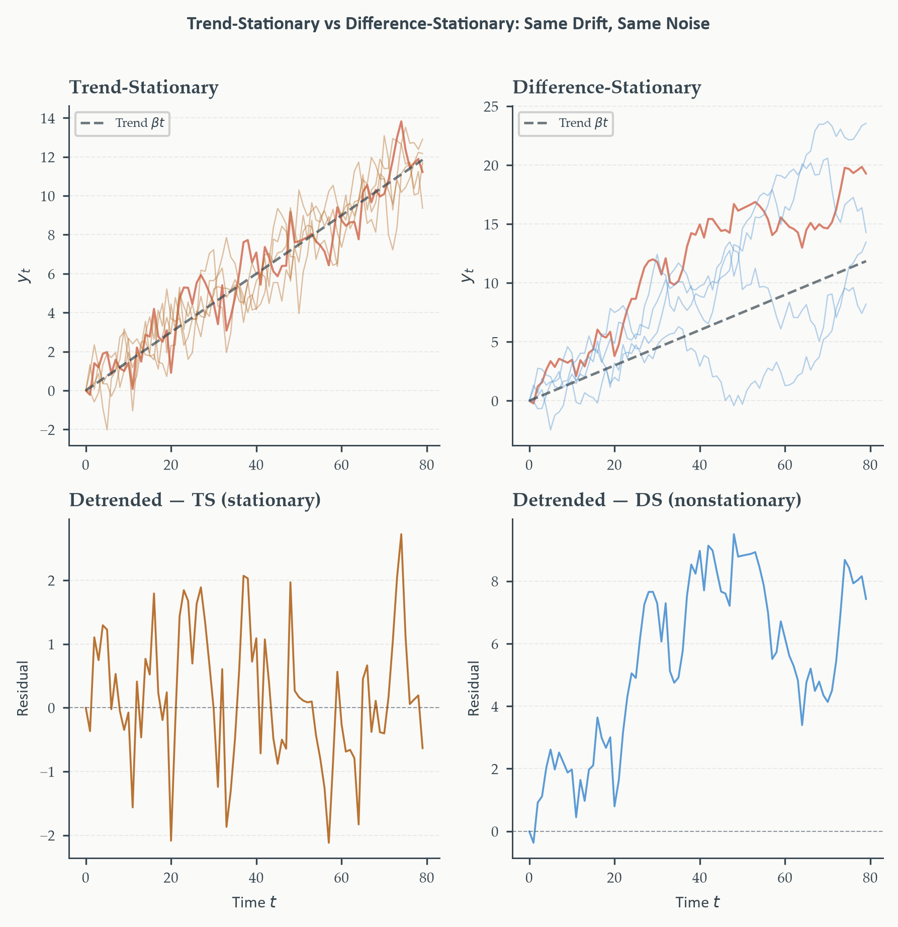
The two processes can look remarkably similar on a single realisation — which
is precisely why formal testing is necessary. The figure below simulates five
paths of each type with the same drift and noise variance. The difference only
becomes apparent over many realisations: trend-stationary paths hug the trend
line and return to it after shocks; difference-stationary paths diverge
permanently and spread ever wider.
```{python}
#| label: fig-ts-vs-ds
#| fig-cap: "Trend-stationary (left) vs difference-stationary (right), five
#| paths each, $T = 80$, same drift and noise variance. Top row: both
#| processes look similar on a single realisation — both trend upward with
#| fluctuations around the trend line (dashed). The difference only becomes
#| apparent across realisations: trend-stationary paths hug the trend and
#| return to it after shocks; difference-stationary paths diverge permanently.
#| Bottom row: residuals after removing the OLS-estimated linear trend.
#| Bottom-left: detrending works for the trend-stationary process — residuals
#| are stationary and fluctuate around zero. Bottom-right: detrending *fails*
#| for the difference-stationary process — the residuals still wander without
#| mean-reversion, because OLS detrending cannot remove a stochastic trend.
#| This is the key diagnostic: if detrended residuals look like the bottom-right
#| panel, the series is difference-stationary and differencing — not detrending
#| — is the correct treatment."
#| fig-width: 6
#| fig-height: 6
#| code-fold: true
#| code-summary: "Show code — trend-stationary vs difference-stationary"
rng_td = np.random.default_rng(seed=123)
T_td   = 80
N_td   = 5
alpha  = 0.0
beta   = 0.15    # drift / trend slope
sig    = 1.0     # noise std

t_axis  = np.arange(T_td)
trend   = alpha + beta * t_axis

fig, axes = plt.subplots(2, 2, figsize=(6, 6))

ts_resid_one = None
ds_resid_one = None

for i in range(N_td):
    eps = rng_td.standard_normal(T_td) * sig

    # Trend-stationary: y_t = alpha + beta*t + u_t, u_t AR(1) with rho=0.5
    u = np.zeros(T_td)
    for t in range(1, T_td):
        u[t] = 0.5 * u[t-1] + eps[t]
    y_ts = trend + u

    # Difference-stationary: delta y_t = beta + eps_t  (random walk with drift)
    y_ds = np.zeros(T_td)
    y_ds[0] = trend[0]
    for t in range(1, T_td):
        y_ds[t] = beta + y_ds[t-1] + eps[t]

    col_a = EO_COPPER if i > 0 else EO_TERRACOTTA
    col_b = EO_SKYBLUE if i > 0 else EO_TERRACOTTA
    lw    = 0.6 if i > 0 else 1.0
    al    = 0.45 if i > 0 else 0.9

    axes[0, 0].plot(t_axis, y_ts, color=col_a, lw=lw, alpha=al)
    axes[0, 1].plot(t_axis, y_ds, color=col_b, lw=lw, alpha=al)

    if i == 0:
        ts_resid_one = u
        ds_resid_one = y_ds - trend   # deviation from OLS trend

# Trend line and labels
for ax, title in [(axes[0,0], "Trend-Stationary"),
                  (axes[0,1], "Difference-Stationary")]:
    ax.plot(t_axis, trend, color=EO_CHARCOAL, lw=1.2,
            ls="--", alpha=0.7, label="Trend $\\beta t$")
    ax.set_title(title)
    ax.set_ylabel("$y_t$")
    ax.legend(fontsize=6)
    eo_style_ax(ax)

# Residuals after removing the linear trend
for ax, resid, title, color in [
    (axes[1,0], ts_resid_one, "Detrended — TS (stationary)",    EO_COPPER),
    (axes[1,1], ds_resid_one, "Detrended — DS (nonstationary)", EO_SKYBLUE),
]:
    ax.plot(t_axis, resid, color=color, lw=0.9)
    ax.axhline(0, color=EO_CHARCOAL, lw=0.5, ls="--", alpha=0.5)
    ax.set_title(title)
    ax.set_ylabel("Residual")
    ax.set_xlabel("Time $t$")
    eo_style_ax(ax)

eo_suptitle(fig, "Trend-Stationary vs Difference-Stationary: Same Drift, Same Noise")
fig.tight_layout()
plt.show()
```
### ARIMA($p$,1,$q$) Is ARMA($p$,$q$) on the Differences
Once $d$ is determined, the connection to Chapter 3 is direct and important.
For $d = 1$, let $w_t = \Delta y_t = y_t - y_{t-1}$. Then equation (4.6) becomes:
$$\phi(L)\,w_t = \mu^* + \theta(L)\,\varepsilon_t \tag{4.6a}$$
This is exactly an ARMA($p$,$q$) model for $w_t$ — the differenced series.
The ARIMA($p$,1,$q$) model for $y_t$ and the ARMA($p$,$q$) model for
$\Delta y_t$ are the same model, just written in terms of different variables.
This equivalence means the complete Box-Jenkins workflow from Chapter 3
applies directly to $\Delta y_t$. The only genuinely new steps are (1)
determining $d$ before the workflow begins, and (2) reconstructing level
forecasts from the forecasts of differences at the end.
::: {.callout-note}
## The ARIMA Workflow: Four Steps
**Step 1 — Determine $d$:** Run ADF and KPSS on the level series.
- If both agree ($I(1)$): set $d = 1$ and work with $\Delta y_t$
- If ADF and KPSS disagree (both reject): suspect a structural break rather
than a pure unit root — investigate subsamples before differencing
- Check $d = 2$ only if $\Delta y_t$ is still visibly nonstationary;
for most economic series $d = 1$ suffices
**Step 2 — Identify $(p,q)$ via Box-Jenkins:** Compute the ACF and PACF of
$\Delta^d y_t$ and apply the Chapter 3 identification table.
- Include a drift term if the level series trends — the mean of $\Delta^d y_t$
should be visibly nonzero
- If seasonal spikes appear at lags $s, 2s, \ldots$, move to SARIMA
identification (Section 4.5) before selecting $(p,q)$
**Step 3 — Estimate and diagnose:** Fit ARIMA$(p,d,q)$ by MLE. Inspect
residual ACF/PACF and the Ljung-Box test exactly as in Chapter 3.
- If Ljung-Box rejects but all residual autocorrelations are below 0.05
in magnitude, the rejection is likely a large-$T$ artefact — assess
economic significance, not just statistical significance
- If significant structure remains at seasonal lags, extend to SARIMA;
at non-seasonal lags, increase $p$ or $q$ and re-diagnose
**Step 4 — Forecast and reconstruct levels:** Produce $h$-step forecasts.
- `statsmodels` reconstructs levels automatically with `order=(p,1,q)` —
`get_forecast()` output is already in level units
- If fitting ARMA directly on $\Delta y_t$, reconstruct manually:
`y_T + fc_delta.cumsum()`
- Prediction intervals widen at rate $\sqrt{h}$ — faster than stationary
ARMA — because uncertainty accumulates without mean-reversion to bound it
:::
### Estimation
Since ARIMA($p$,1,$q$) on $y_t$ is ARMA($p$,$q$) on $\Delta y_t$, estimation
is exactly the MLE procedure from Chapter 3, Section 3.7 — applied to the
differenced series. No new theory is needed. In practice, `statsmodels` handles
the differencing transparently: specifying `order=(p, 1, q)` in `ARIMA()`
automatically differences the series before constructing the likelihood, and
the output — coefficients, standard errors, information criteria — is read
exactly as in Chapter 3.
### auto\_arima: A Practical Search Tool
Choosing $(p,d,q)$ by the manual Box-Jenkins workflow — examine ACF/PACF,
select candidate orders, fit, diagnose, revise — is the principled approach
and the one that builds genuine understanding. In practice, researchers often
use **auto-ARIMA** to search over a grid of $(p,q)$ orders for a given $d$
and select by information criteria. The `pmdarima` library provides this:
```python
from pmdarima import auto_arima
model = auto_arima(y, d=1, max_p=4, max_q=4,
                   information_criterion='bic',
                   stepwise=True, seasonal=False)
```
The `stepwise=True` option uses a stepwise search (Hyndman and Khandakar,
2008) rather than exhaustive grid search, making it feasible for large grids.
Starting from ARIMA(2,1,2), it tests neighbouring specifications and moves
in the direction of improving BIC until no further improvement is possible.
### Python: Identifying and Estimating an ARIMA for Log SA GDP
We now apply the full ARIMA workflow to log SA real GDP. The unit root tests
confirmed $d = 1$. We examine the ACF and PACF of the first-differenced series
(GDP growth) to determine $p$ and $q$, then estimate, use `auto_arima` as a
cross-check, and diagnose.
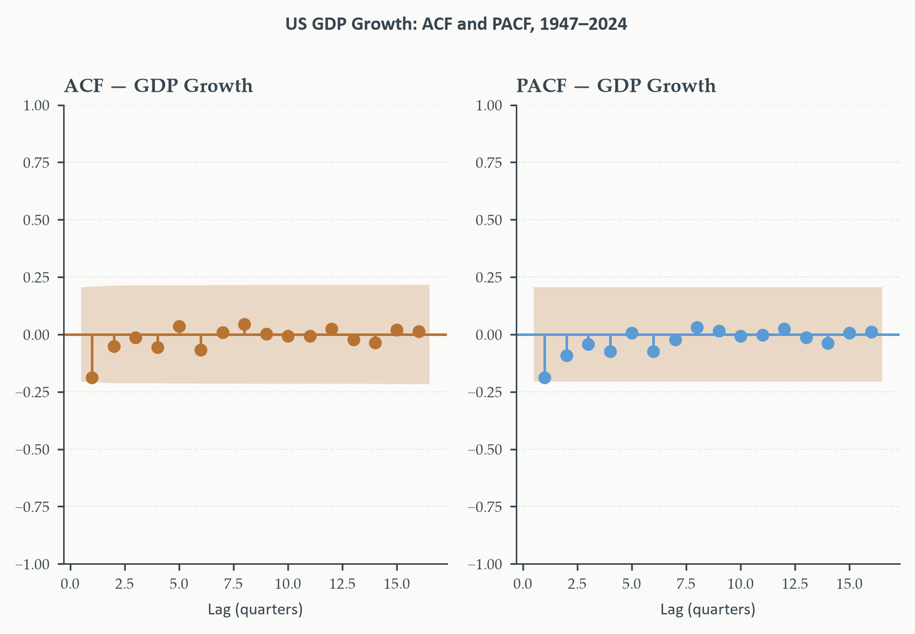
```{python}
#| label: fig-gdp-growth-acfpacf
#| fig-cap: "ACF and PACF of quarterly US GDP growth (log-differenced SA
#| real GDP), 1947Q2–2024Q3. The ACF tails off gradually; the PACF shows
#| a significant spike at lag 1 and possibly lag 2, with values inside
#| the band thereafter. This pattern is broadly consistent with an AR(1)
#| or AR(2) process for GDP growth — equivalently, an ARIMA(1,1,0) or
#| ARIMA(2,1,0) for the level. The MA identification is less clear,
#| suggesting an ARMA(p,q) structure that information criteria will
#| help resolve."
#| fig-width: 6
#| fig-height: 4
#| code-fold: true
#| code-summary: "Show code — GDP growth ACF/PACF"
fig, axes = plt.subplots(1, 2, figsize=(6, 4))

gr_clean = gdp["GDP Growth"].dropna()

ax = axes[0]
plot_acf(gr_clean, lags=16, ax=ax,
         color=EO_COPPER, vlines_kwargs={"colors": EO_COPPER},
         title="ACF — GDP Growth", zero=False, alpha=0.05)
ax.set_xlabel("Lag (quarters)")
eo_style_ax(ax)
for line in ax.lines:
    if line.get_linestyle() == "--":
        line.set_color(EO_TERRACOTTA)
        line.set_linewidth(0.8)

ax = axes[1]
plot_pacf(gr_clean, lags=16, ax=ax,
          color=EO_SKYBLUE, vlines_kwargs={"colors": EO_SKYBLUE},
          title="PACF — GDP Growth", zero=False, alpha=0.05)
ax.set_xlabel("Lag (quarters)")
eo_style_ax(ax)
for line in ax.lines:
    if line.get_linestyle() == "--":
        line.set_color(EO_TERRACOTTA)
        line.set_linewidth(0.8)

eo_suptitle(fig, "US GDP Growth: ACF and PACF, 1947–2024")
fig.tight_layout()
plt.show()
```
The ACF and PACF of GDP growth suggest autoregressive structure at short lags,
consistent with ARIMA(1,1,0) or ARIMA(2,1,0) as starting candidates. We now
fit a grid of ARIMA models on log SA GDP and compare by information criteria,
then use `auto_arima` as a cross-check.
```{python}
#| label: install-pmdarima
#| include: false
import subprocess
subprocess.run(["pip", "install", "pmdarima", "--quiet",
"--break-system-packages"], check=True)
```
```{python}
#| label: tbl-arima-ic
#| code-fold: true
#| code-summary: "Show code — ARIMA model selection"
from pmdarima import auto_arima as pm_auto_arima

# ── Restrict to pre-COVID sample ──────────────────────────────────────────────
# gdp_level_pre defined earlier in fig-spurious cell; redefined here
# for clarity and to ensure it is in scope for all subsequent cells.
gdp_level     = gdp["Log SA"].dropna()
gdp_level_pre = gdp_level[:"2019-12-31"]

results = []
for p in range(0, 4):
    for q in range(0, 4):
        if p == 0 and q == 0:
            continue
        try:
            mod = ARIMA(gdp_level_pre, order=(p, 1, q)).fit()
            results.append({
                "Model":  f"ARIMA({p},1,{q})",
                "Params": p + q + 2,
                "AIC":    round(mod.aic, 1),
                "BIC":    round(mod.bic, 1),
                "HQ":     round(mod.hqic, 1),
            })
        except Exception:
            pass

ic_df = (pd.DataFrame(results)
           .sort_values("BIC")
           .reset_index(drop=True))

col_w = 14
mnames = ["Model", "Params", "AIC", "BIC", "HQ"]

header = "".join(f"{m:>{col_w}}" for m in mnames)
print(header)
print("─" * (col_w * len(mnames)))
for _, row in ic_df.head(8).iterrows():
    line = (f"{row['Model']:>{col_w}}"
            f"{int(row['Params']):>{col_w}}"
            f"{row['AIC']:>{col_w}.1f}"
            f"{row['BIC']:>{col_w}.1f}"
            f"{row['HQ']:>{col_w}.1f}")
    print(line)

# ── auto_arima cross-check ─────────────────────────────────────────────────────
print("\n" + "─" * 50)
print("auto_arima cross-check (BIC, stepwise, 1947–2019):")
auto_mod = pm_auto_arima(gdp_level_pre, d=1, max_p=4, max_q=4,
                          information_criterion="bic",
                          stepwise=True, seasonal=False,
                          suppress_warnings=True, error_action="ignore")
print(f"  Selected: ARIMA{auto_mod.order}")
print(f"  AIC: {auto_mod.aic():.1f}  BIC: {auto_mod.bic():.1f}")
```
*Top ARIMA specifications for log SA real GDP by BIC, sorted ascending.
`auto_arima` (BIC, stepwise) cross-check shown below the table.*
::: {.callout-warning icon=false}
## auto\_arima Is a Search Tool, Not a Black Box
`auto_arima` is useful for quickly surveying candidate specifications, but
it has important limitations. First, it relies on information criteria and
therefore inherits all their limitations — in particular, BIC will
favour parsimony and may miss important structure in small samples. Second,
stepwise search is not exhaustive and can miss the global optimum. Third,
and most importantly, it bypasses the diagnostic step: a model selected by
`auto_arima` must still be checked against the data with residual ACF/PACF
plots and the Ljung-Box test. Treating the auto-selected model as the final
answer without diagnostics is the most common misuse. Use `auto_arima` to
generate candidate specifications, then validate them manually.
:::
Two things to note when reading the output. First, `auto_arima` may report
a different BIC value for the same model order than the grid search — and
may even select a different order. This reflects differences in how
`pmdarima` and `statsmodels` handle the constant term, initialise the
presample, and scale the log-likelihood. IC values are only comparable within
the same estimation framework. When both methods agree on the order, the
discrepancy is cosmetic; when they disagree, fit both and let residual
diagnostics decide.
Second, BIC and HQ favour parsimony — likely ARIMA(1,1,0) or ARIMA(1,1,1)
— reflecting the mild AR(1) structure visible in the GDP growth ACF/PACF.
AIC may select a richer model. We fit the BIC-preferred specification and
run diagnostics.
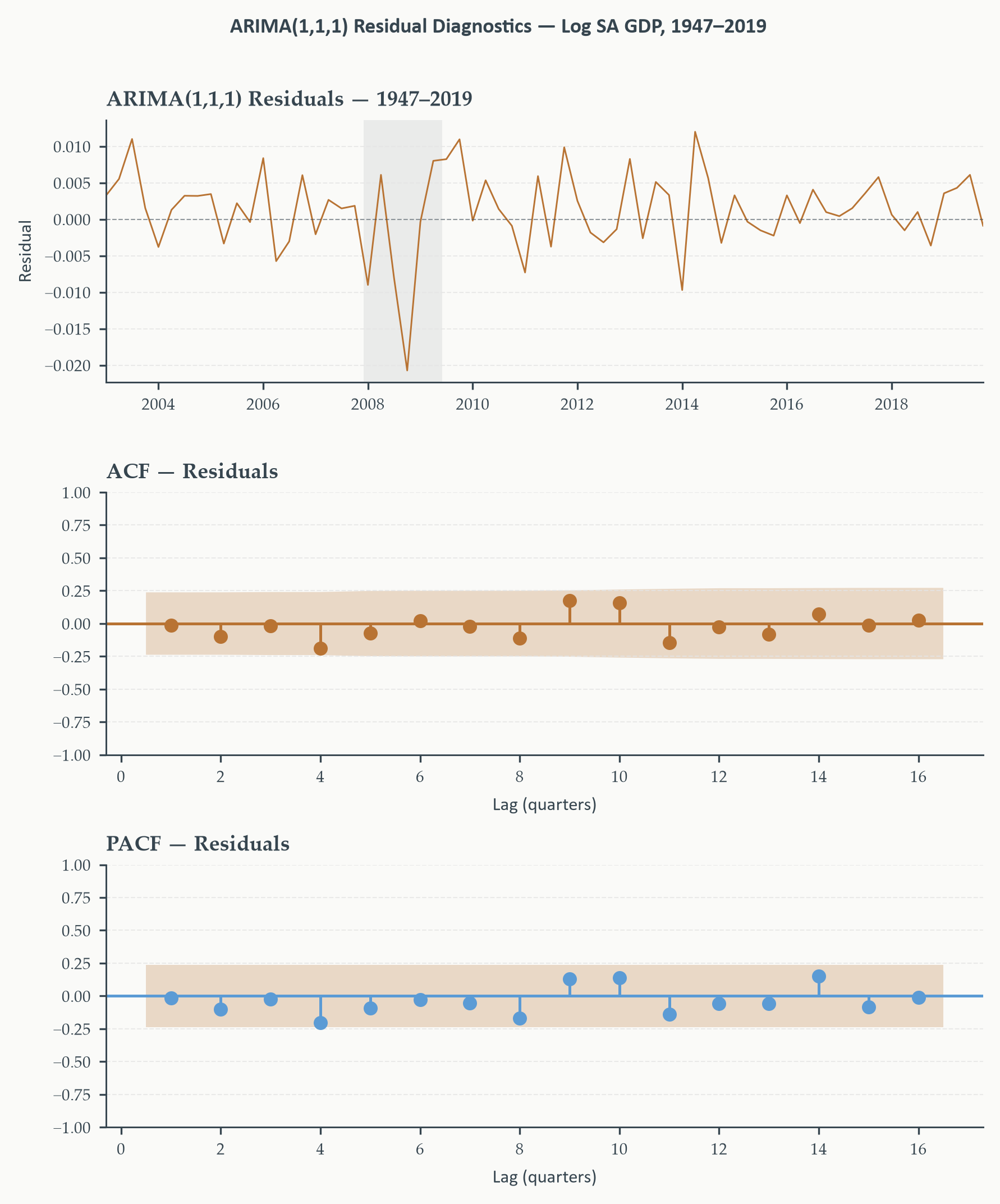
```{python}
#| label: fig-arima-diagnostics
#| fig-cap: "ARIMA residual diagnostics for log SA real GDP, 1947–2019.
#| Top: residual time series with NBER recessions shaded — no dominant
#| outlier distorts the scale. Middle: residual ACF. Bottom: residual PACF.
#| A well-specified model shows no systematic structure beyond sampling noise."
#| fig-width: 6
#| fig-height: 7
#| code-fold: true
#| code-summary: "Show code — ARIMA diagnostics"
import re
best_order = ic_df.loc[ic_df["BIC"].idxmin(), "Model"]
match   = re.search(r"ARIMA\((\d+),1,(\d+)\)", best_order)
p_best  = int(match.group(1))
q_best  = int(match.group(2))

mod_best    = ARIMA(gdp_level_pre, order=(p_best, 1, q_best)).fit()
# Drop first few residuals which can be erratic due to presample initialisation
resid_arima = mod_best.resid.dropna().iloc[4:]

print(f"Fitting: ARIMA({p_best},1,{q_best}) on 1947–2019")
print(mod_best.summary())

fig, axes = plt.subplots(3, 1, figsize=(6, 7))

ax = axes[0]
ax.plot(resid_arima.index, resid_arima.values,
        color=EO_COPPER, lw=0.7)
ax.axhline(0, color=EO_CHARCOAL, lw=0.5, ls="--", alpha=0.5)
shade_recessions(ax)
ax.set_xlim(resid_arima.index[0], resid_arima.index[-1])
ax.set_title(f"ARIMA({p_best},1,{q_best}) Residuals — 1947–2019")
ax.set_ylabel("Residual")
eo_style_ax(ax)

ax = axes[1]
plot_acf(resid_arima, lags=16, ax=ax,
         color=EO_COPPER, vlines_kwargs={"colors": EO_COPPER},
         title="ACF — Residuals", zero=False, alpha=0.05)
ax.set_xlabel("Lag (quarters)")
eo_style_ax(ax)
for line in ax.lines:
    if line.get_linestyle() == "--":
        line.set_color(EO_TERRACOTTA)
        line.set_linewidth(0.8)

ax = axes[2]
plot_pacf(resid_arima, lags=16, ax=ax,
          color=EO_SKYBLUE, vlines_kwargs={"colors": EO_SKYBLUE},
          title="PACF — Residuals", zero=False, alpha=0.05)
ax.set_xlabel("Lag (quarters)")
eo_style_ax(ax)
for line in ax.lines:
    if line.get_linestyle() == "--":
        line.set_color(EO_TERRACOTTA)
        line.set_linewidth(0.8)

eo_suptitle(fig,
    f"ARIMA({p_best},1,{q_best}) Residual Diagnostics — Log SA GDP, 1947–2019")
fig.tight_layout()
plt.show()
```
Before running diagnostics, a note on sample choice. We restrict estimation to
1947–2019 throughout this section. The COVID-19 contraction of 2020Q2 — a
loss of nearly 10% of GDP in a single quarter — is a pandemic-driven event
with no counterpart in the postwar data. Fitting an ARIMA model on the full
sample would give this single observation enormous leverage over the parameter
estimates and dominate every residual plot, obscuring the model's actual
performance on normal business cycle dynamics. This is the same logic applied
to the ICSA series in Chapter 3: when an outlier reflects a structural break
or an extraordinary event rather than model misspecification, restricting the
estimation sample is the honest choice. Chapter 6 provides the formal tools —
Chow tests and Bai-Perron — to test whether such restrictions are justified.
An alternative to sample restriction is to include an **additive outlier dummy**
directly in the model. A dummy variable equal to 1 for the COVID quarter and
zero otherwise can be added as an exogenous regressor via the `exog` argument
in `statsmodels`' `ARIMA` or `SARIMAX`:
```python
covid_dummy = (gdp_level.index == "2020-04-01").astype(float)
mod = ARIMA(gdp_level, order=(p, 1, q),
            exog=covid_dummy.values.reshape(-1, 1)).fit()
```
This allows the full sample to be used while absorbing the outlier's distorting
effect on the parameter estimates. Multiple dummies handle multiple outlier
quarters. The estimated dummy coefficient measures the size of the outlier
directly — if it is large and significant, restricting the sample was the right
instinct. This approach connects to the structural break framework in Chapter 6,
where dummies for known break dates are a standard modelling tool.
## Forecasting with ARIMA {#sec-arimaforecast}
### How Integration Changes the Forecast
An ARMA model forecasts levels directly — the $h$-step forecast pulls toward
the unconditional mean as the horizon grows, and prediction intervals eventually
plateau at the unconditional variance. An ARIMA model works differently. Because
the model is defined on the differences, it fundamentally **forecasts changes**,
not levels. Level forecasts are then recovered by accumulating those predicted
changes from the last observed level — exactly the reconstruction step in the
ARIMA workflow. This indirect path from changes to levels is what makes ARIMA
forecasts behave differently from ARMA forecasts in two important ways.
**Forecasts do not mean-revert.** The ARMA forecast of $\Delta y_t$ converges
to the estimated drift $\hat\mu$ at long horizons, and accumulating a constant
change per period produces a **linear trend** in the level forecast — not a
return to any fixed level. For the simplest case, ARIMA(0,1,0) with drift:
$$\hat{y}_{T+h|T} = y_T + h\hat\mu \tag{4.8}$$
The forecast is anchored to where the series is *today*, not to any historical
mean. A permanent shock shifts the entire forecast path permanently upward or
downward.
**Prediction intervals widen without bound.** Each accumulated step adds
independent forecast uncertainty. The standard deviation of the $h$-step
level forecast error grows as $\sqrt{h}$ — the same $\sqrt{t}$ envelope
visible in the random walk paths of Section 4.1 — not bounded by any finite
unconditional variance.
::: {.callout-note}
## ARIMA vs ARMA Forecasting: The Key Difference
| Feature | ARMA (stationary) | ARIMA ($d=1$) |
|:--------|:-----------------|:--------------|
| Forecasts what? | Levels directly | Changes; levels by accumulation |
| Long-run forecast | Converges to $\hat\mu$ | Linear trend extrapolation |
| Interval width | Plateaus at $\sigma_y$ | Grows as $\sqrt{h}$, unbounded |
| Anchor | Unconditional mean | Current level $y_T$ |
:::
### Python: ARIMA Forecasts for Log SA GDP
We produce $h = 20$ quarter-ahead forecasts (five years) from the selected
ARIMA model, plotting both a 95% interval and a fan chart. The growing interval
width is one of the key visual features that distinguishes ARIMA from ARMA
forecasts.
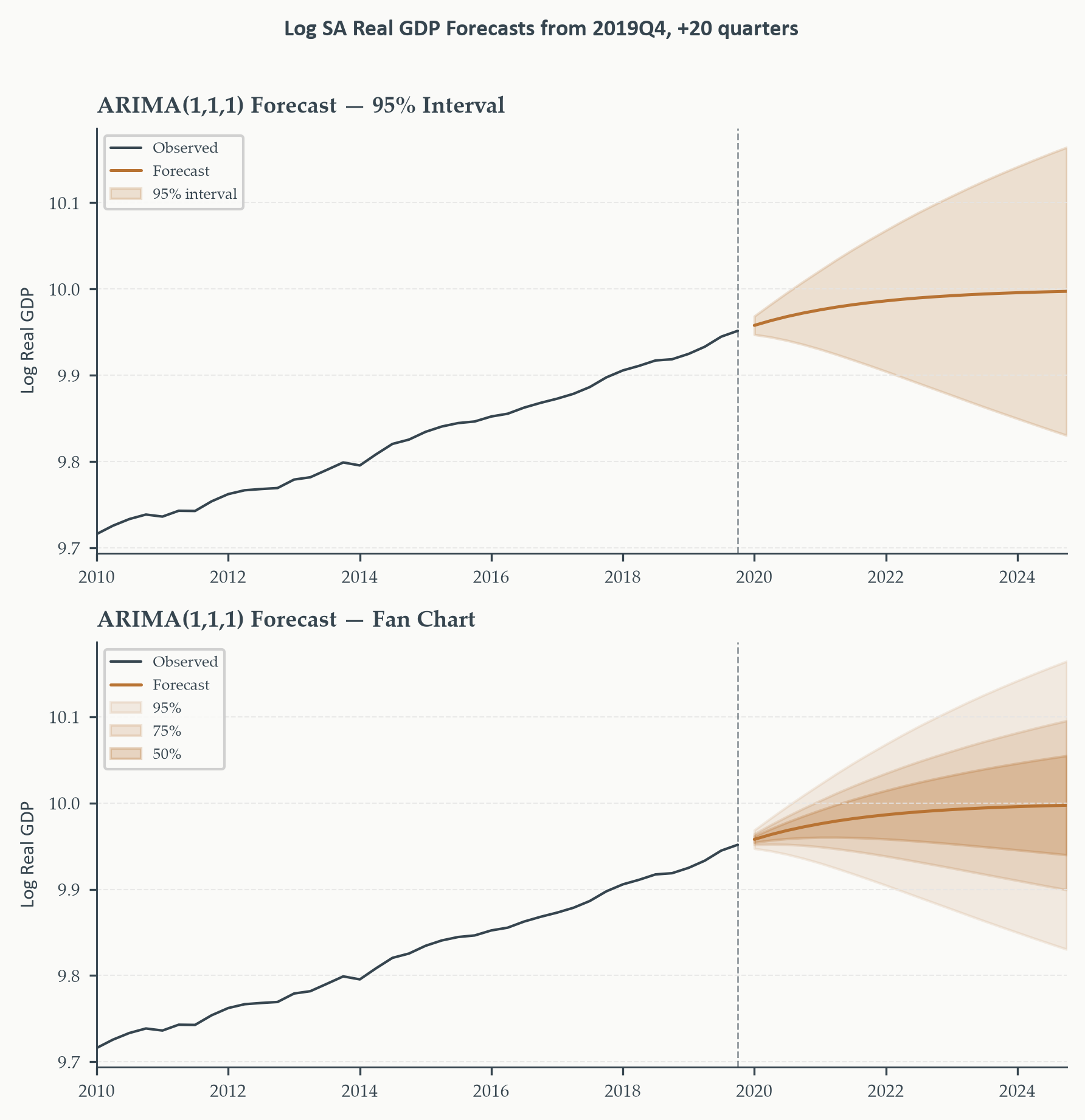
```{python}
#| label: fig-arima-forecast
#| fig-cap: "ARIMA forecasts for log SA real GDP, 20 quarters ahead from
#| 2024Q3. Top: point forecast (copper) with 95% prediction interval
#| (shaded), overlaid on the last 10 years of observed data (charcoal).
#| The forecast extrapolates the recent growth trend; the interval widens
#| at rate $\\sqrt{h}$, reflecting the unit root in the level. Bottom:
#| fan chart showing 50%, 75%, and 95% intervals — the widening fan is
#| more dramatic than for stationary ARMA forecasts because uncertainty
#| accumulates without the mean-reversion dampening that bounds interval
#| width in the stationary case."
#| fig-width: 6
#| fig-height: 6
#| code-fold: true
#| code-summary: "Show code — ARIMA forecasts"
h = 20   # quarters ahead

fc       = mod_best.get_forecast(steps=h)
fc_mean  = fc.predicted_mean
fc_ci95  = fc.conf_int(alpha=0.05)
fc_ci75  = fc.conf_int(alpha=0.25)
fc_ci50  = fc.conf_int(alpha=0.50)

# Last 10 years of pre-COVID observed data for context
obs_tail = gdp_level_pre.iloc[-40:]

fig, axes = plt.subplots(2, 1, figsize=(6, 6), sharex=False)

# ── Panel 1: 95% interval ─────────────────────────────────────────────────────
ax = axes[0]
ax.plot(obs_tail.index, obs_tail.values,
        color=EO_CHARCOAL, lw=1.0, label="Observed")
ax.plot(fc_mean.index, fc_mean.values,
        color=EO_COPPER, lw=1.2, label="Forecast")
ax.fill_between(fc_ci95.index,
                fc_ci95.iloc[:, 0], fc_ci95.iloc[:, 1],
                color=EO_COPPER, alpha=0.20, label="95% interval")
ax.axvline(obs_tail.index[-1], color=EO_CHARCOAL,
           lw=0.7, ls="--", alpha=0.5)
ax.set_xlim(obs_tail.index[0], fc_ci95.index[-1])
ax.set_title(f"ARIMA({p_best},1,{q_best}) Forecast — 95% Interval")
ax.set_ylabel("Log Real GDP")
ax.legend(fontsize=6)
eo_style_ax(ax)

# ── Panel 2: fan chart ────────────────────────────────────────────────────────
ax = axes[1]
ax.plot(obs_tail.index, obs_tail.values,
        color=EO_CHARCOAL, lw=1.0, label="Observed")
ax.plot(fc_mean.index, fc_mean.values,
        color=EO_COPPER, lw=1.2, label="Forecast")
ax.fill_between(fc_ci95.index,
                fc_ci95.iloc[:, 0], fc_ci95.iloc[:, 1],
                color=EO_COPPER, alpha=0.12, label="95%")
ax.fill_between(fc_ci75.index,
                fc_ci75.iloc[:, 0], fc_ci75.iloc[:, 1],
                color=EO_COPPER, alpha=0.18, label="75%")
ax.fill_between(fc_ci50.index,
                fc_ci50.iloc[:, 0], fc_ci50.iloc[:, 1],
                color=EO_COPPER, alpha=0.28, label="50%")
ax.axvline(obs_tail.index[-1], color=EO_CHARCOAL,
           lw=0.7, ls="--", alpha=0.5)
ax.set_xlim(obs_tail.index[0], fc_ci95.index[-1])
ax.set_title(f"ARIMA({p_best},1,{q_best}) Forecast — Fan Chart")
ax.set_ylabel("Log Real GDP")
ax.legend(fontsize=6)
eo_style_ax(ax)

end_yr = gdp_level_pre.index[-1].year
end_q  = gdp_level_pre.index[-1].quarter
eo_suptitle(fig,
    f"Log SA Real GDP Forecasts from {end_yr}Q{end_q}, +{h} quarters")
fig.tight_layout()
plt.show()
```
Three features of the forecast deserve comment.
**The drift term drives the long-run forecast.** The point forecast extrapolates
at roughly the historical average growth rate of log GDP. Unlike the ARMA
forecast in Chapter 3 which pulled toward a fixed unconditional mean, this
forecast has no fixed attractor — it projects forward along the current
trajectory.
**The interval widens much faster than in Chapter 3.** Compare the fan chart
here to the ICSA fan chart in Chapter 3: the ICSA intervals eventually plateaued
as the forecast converged to the unconditional mean. Here there is no plateau.
By quarter 20, the 95% interval spans a substantial range of log GDP values,
reflecting five years of accumulated uncertainty with no mean-reversion to
bound it.
**The $\sqrt{h}$ envelope.** The standard deviation of the $h$-step forecast
error is approximately $\hat\sigma_\Delta\sqrt{h}$, where
$\hat\sigma_\Delta$ is the estimated standard deviation of quarterly GDP
growth. The interval width grows proportionally to $\sqrt{h}$: doubling the
horizon increases the interval width by factor $\sqrt{2} \approx 1.41$, not
by factor 2. The fan chart visualises this — the shaded bands widen noticeably
but not explosively over five years.
### Reconstructing Level Forecasts from Forecasts of Differences
Since ARIMA($p$,1,$q$) on $y_t$ is ARMA($p$,$q$) on $\Delta y_t$, the model
directly produces forecasts of *changes* — quarterly growth rates in the GDP
case. The level forecast is recovered by cumulating those predicted changes
from the last observed level:
$$\hat{y}_{T+h|T} = y_T + \sum_{j=1}^{h} \hat{\Delta y}_{T+j|T} \tag{4.10}$$
`statsmodels`' `get_forecast()` performs this reconstruction automatically when
the model is specified with `order=(p, 1, q)` — the output is already in log
level units. Students who fit an ARMA directly on the differenced series and
want level forecasts must apply equation (4.10) manually: take the last
observed level, add the first predicted growth rate to get $\hat{y}_{T+1|T}$,
add the second to get $\hat{y}_{T+2|T}$, and so on. In Python this is a
one-liner: `y_T + fc_delta.cumsum()`. The widening prediction intervals in the
level come from this accumulation — each additional step adds independent
forecast uncertainty that does not cancel, producing the $\sqrt{h}$ growth in
interval width established in equation (4.9).
## Seasonality and SARIMA {#sec-sarima}
### Two Kinds of Seasonality
Many economic time series repeat a recognisable pattern at regular intervals.
Retail sales surge in December. Construction activity peaks in summer and troughs
in winter. Jobless claims spike in January as holiday workers are laid off.
Agricultural output follows the growing season. These patterns are not random —
they reflect genuine, calendar-driven regularities in economic behaviour. How
we model them depends on their nature.
**Deterministic seasonality** is a fixed, repeating pattern with constant
amplitude. If December retail sales are always $k$ percent higher than the annual
average, regardless of the overall state of the economy, a set of seasonal dummy
variables — one for each period of the year minus one — captures this exactly.
The seasonal pattern does not evolve over time; it is anchored to specific calendar
positions.
**Stochastic seasonality** is a seasonal pattern whose amplitude and shape change
over time. The Christmas peak may be stronger in boom years and weaker in
recessions. The winter construction trough may shift as climate and building
practices evolve. Seasonal dummies cannot capture this time-variation; what is
needed is a model that allows the seasonal pattern itself to be an integrated
process — one that drifts over time rather than repeating identically.
The SARIMA framework handles stochastic seasonality through **seasonal
differencing**: comparing each observation to the same period in the previous
year, rather than to the previous period. This removes a slowly-evolving seasonal
mean in the same way that regular differencing removes a slowly-evolving level.
### The Seasonal Difference Operator
For a series observed $s$ times per year (quarterly: $s=4$; monthly: $s=12$;
weekly: $s=52$), the **seasonal difference operator** is:
$$\Delta_s = 1 - L^s, \qquad \Delta_s y_t = y_t - y_{t-s} \tag{4.11}$$
For quarterly data, $\Delta_4 y_t = y_t - y_{t-4}$ compares this quarter to the
same quarter last year — removing the annual seasonal pattern directly. If the
seasonal pattern is deterministic and constant, one seasonal difference suffices
to remove it. If it is stochastic and evolving, the seasonal difference may itself
need regular differencing.
The seasonal difference operator has a unit root at the seasonal frequency: the
polynomial $1 - L^s$ has $s$ roots of unit modulus, evenly spaced around the
unit circle at angles $2\pi k/s$ for $k = 0, 1, \ldots, s-1$. Seasonal
differencing removes all $s$ of these seasonal unit roots simultaneously. This
is analogous to regular differencing removing the unit root at $z = 1$ — but
now applied at every seasonal frequency.
### The SARIMA$(p,d,q)(P,D,Q)_s$ Model
The **Seasonal ARIMA** model extends ARIMA by adding a second layer of AR and
MA terms that operate at the seasonal lag $s$ rather than the unit lag. Before
writing the compact polynomial form, it helps to see the model in expanded
notation for the quarterly case ($s = 4$, $d = D = 1$).
The model applies two differencing operations to $y_t$. First, the **seasonal
difference** $\Delta_4 y_t = y_t - y_{t-4}$ compares each quarter to the same
quarter of the previous year, removing the stochastic seasonal pattern. Second,
the **regular difference** $\Delta(\Delta_4 y_t) = \Delta_4 y_t - \Delta_4
y_{t-1}$ removes the stochastic trend. To keep the equation readable, define:
$$w_t = \Delta_4\Delta y_t = (y_t - y_{t-4}) - (y_{t-1} - y_{t-5})$$
This is the doubly-differenced series — seasonally and trend adjusted. The
SARIMA model is then an ARMA on $w_t$ with both regular and seasonal lag
terms:
$$\begin{aligned}
w_t = \mu^*
&+ \underbrace{\phi_1 w_{t-1} + \cdots + \phi_p w_{t-p}}_{\text{non-seasonal AR}(p)}
+ \underbrace{\Phi_1 w_{t-4} + \cdots + \Phi_P w_{t-4P}}_{\text{seasonal AR}(P)} \\
&+ \underbrace{\varepsilon_t + \theta_1\varepsilon_{t-1} + \cdots + \theta_q\varepsilon_{t-q}}_{\text{non-seasonal MA}(q)}
+ \underbrace{\Theta_1\varepsilon_{t-4} + \cdots + \Theta_Q\varepsilon_{t-4Q}}_{\text{seasonal MA}(Q)}
\end{aligned}
\tag{4.11}$$
where $w_t = \Delta_4\Delta y_t$. The non-seasonal AR and MA terms capture
quarter-to-quarter dynamics at adjacent lags; the seasonal terms capture
year-over-year dynamics at lags that are multiples of 4. In compact lag
polynomial notation:
$$\Phi(L^s)\,\phi(L)\,(1-L^s)^D\,(1-L)^d\,y_t
= \mu^* + \Theta(L^s)\,\theta(L)\,\varepsilon_t \tag{4.12}$$
where the notation distinguishes two components:
::: {.callout-note}
## Definition 4.5 — SARIMA$(p,d,q)(P,D,Q)_s$
**Non-seasonal component** (operates at lag 1):
- $\phi(L) = 1 - \phi_1 L - \cdots - \phi_p L^p$: AR polynomial of order $p$
- $(1-L)^d$: $d$ regular differences
- $\theta(L) = 1 + \theta_1 L + \cdots + \theta_q L^q$: MA polynomial of order $q$
**Seasonal component** (operates at lag $s$):
- $\Phi(L^s) = 1 - \Phi_1 L^s - \cdots - \Phi_P L^{Ps}$: seasonal AR of order $P$
- $(1-L^s)^D$: $D$ seasonal differences
- $\Theta(L^s) = 1 + \Theta_1 L^s + \cdots + \Theta_Q L^{Qs}$: seasonal MA of order $Q$
The model requires all characteristic roots of $\phi(L)$, $\Phi(L^s)$,
$\theta(L)$, and $\Theta(L^s)$ to lie inside the unit circle for stationarity
and invertibility. In practice, $D \leq 1$ and $d \leq 1$ for most economic series.
:::
The two layers interact multiplicatively. Written out for the common
SARIMA$(1,1,1)(1,1,1)_4$ case:
$$(1 - \phi_1 L)(1 - \Phi_1 L^4)(1-L)(1-L^4)\,y_t
= (1 + \theta_1 L)(1 + \Theta_1 L^4)\,\varepsilon_t$$
The $(1-L)(1-L^4)$ differencing removes both the stochastic trend and the
stochastic seasonal pattern. The AR and MA polynomials then model the remaining
short-run and seasonal autocorrelation structure.
### Why SARIMA and Not SARMA?
A natural question is why the seasonal model includes differencing at all —
why not a stationary SARMA with $d = D = 0$? The answer reflects what we
typically see in economic data. Seasonally unadjusted series like NSA GDP
almost always have *both* a stochastic trend (requiring $d = 1$) and a
stochastic seasonal pattern whose amplitude evolves over time (requiring
$D = 1$). A SARMA model assumes the seasonal pattern repeats identically each
year with constant amplitude — essentially deterministic seasonality — which
is rarely appropriate for macroeconomic data over long samples. Seasonal
adjustment at the data stage (producing the SA series) removes the seasonal
component, reducing SARIMA back to ARIMA. When working with raw NSA series,
SARIMA is the appropriate tool.
### Seasonal ACF/PACF Identification
Just as ARIMA($p$,1,$q$) on $y_t$ is equivalent to ARMA($p$,$q$) on $\Delta y_t$,
the SARIMA$(p,1,q)(P,1,Q)_4$ model on $y_t$ is equivalent to a seasonal ARMA
on the doubly-differenced series $\Delta_4\Delta y_t$. Once both the regular
and seasonal unit roots are removed by differencing, the same Chapter 3
identification logic applies — the only new task is reading both unit lags
and seasonal lags simultaneously.
The identification rules extend naturally to two frequencies: the short-run
lags (1, 2, 3) and the seasonal lags ($s$, $2s$, $3s$). The extended
identification table is:
| Pattern | Suggested specification |
|:--------|:------------------------|
| PACF cuts off after lag $p$; ACF tails off at unit lags | AR($p$) non-seasonal component |
| ACF cuts off after lag $q$; PACF tails off at unit lags | MA($q$) non-seasonal component |
| PACF cuts off after lag $Ps$; ACF tails off at seasonal lags | SAR($P$) seasonal component |
| ACF cuts off after lag $Qs$; PACF tails off at seasonal lags | SMA($Q$) seasonal component |
In practice, $P$ and $Q$ are almost always 0 or 1 for quarterly data, and
$D = 1$ when seasonal differencing is required. Starting from
SARIMA$(1,1,0)(1,1,0)_4$ or SARIMA$(0,1,1)(0,1,1)_4$ and refining by
information criteria is a reliable default strategy for quarterly economic series.
### Python: SARIMA for NSA Real GDP
The NSA (non-seasonally adjusted) real GDP series from Chapter 2 shows pronounced
quarterly seasonality: output is consistently lower in Q1 (winter), rises
through Q2 and Q3, and peaks in Q4. This pattern is stochastic — its amplitude
varies with the business cycle — making SARIMA the appropriate framework.
```{python}
#| label: fig-nsa-gdp
#| fig-cap: "Log NSA real GDP (top) and its seasonal and regular differences
#| $\\Delta_4\\Delta y_t$ (bottom), 1947Q1–2024Q3. The level shows both
#| the upward stochastic trend and the pronounced seasonal swing — the
#| within-year dip in Q1 is visible as a regular sawtooth pattern
#| superimposed on the trend. After applying both seasonal and regular
#| differencing, the series fluctuates around zero with no visible trend
#| or seasonal pattern."
#| fig-width: 6
#| fig-height: 5
#| code-fold: true
#| code-summary: "Show code — NSA GDP and differencing"
gdp_nsa_log = gdp["Log NSA"].dropna()

# Seasonal difference (removes seasonal unit root)
d4_nsa  = gdp_nsa_log.diff(4).dropna()
# Regular + seasonal difference (removes trend and seasonal unit roots)
d1d4_nsa = d4_nsa.diff(1).dropna()

fig, axes = plt.subplots(2, 1, figsize=(6, 5), sharex=False)

ax = axes[0]
ax.plot(gdp_nsa_log.index, gdp_nsa_log.values,
        color=EO_COPPER, lw=0.9)
shade_recessions(ax)
ax.set_xlim(gdp_nsa_log.index[0], gdp_nsa_log.index[-1])
ax.set_title("Log NSA Real GDP — Level")
ax.set_ylabel("Log SAAR billions (2017 $)")
eo_style_ax(ax)

import matplotlib.dates as mdates

ax = axes[1]
ax.plot(d1d4_nsa.index, d1d4_nsa.values,
        color=EO_SKYBLUE, lw=0.8)
ax.axhline(0, color=EO_CHARCOAL, lw=0.5, ls="--", alpha=0.5)
shade_recessions(ax)
ax.set_xlim(d1d4_nsa.index[0], d1d4_nsa.index[-1])
ax.xaxis.set_major_locator(mdates.YearLocator(10))
ax.xaxis.set_major_formatter(mdates.DateFormatter("%Y"))
ax.set_title("$\\Delta_4\\Delta$ Log NSA GDP — Seasonal + Regular Difference")
ax.set_ylabel("Difference")
eo_style_ax(ax)

eo_suptitle(fig, "Log NSA Real GDP: Level and Differenced, 1947–2024")
fig.tight_layout()
plt.show()
```
```{python}
#| label: fig-nsa-acfpacf
#| fig-cap: "ACF and PACF of $\\Delta_4\\Delta$ log NSA real GDP. Unit lags
#| (1, 2, 3) and seasonal lags (4, 8, 12) should both be inspected.
#| Significant spikes at lags 1 and 4 in the ACF and/or PACF signal
#| non-seasonal AR/MA and seasonal AR/MA structure respectively, pointing
#| toward a SARIMA$(p,1,q)(P,1,Q)_4$ specification."
#| fig-width: 6
#| fig-height: 4
#| code-fold: true
#| code-summary: "Show code — seasonal ACF/PACF"
fig, axes = plt.subplots(1, 2, figsize=(6, 4))

ax = axes[0]
plot_acf(d1d4_nsa, lags=16, ax=ax,
         color=EO_COPPER, vlines_kwargs={"colors": EO_COPPER},
         title="ACF — $\\Delta_4\\Delta$ Log NSA GDP",
         zero=False, alpha=0.05)
ax.set_xlabel("Lag (quarters)")
eo_style_ax(ax)
# Mark seasonal lags
for s_lag in [4, 8, 12]:
    ax.axvline(s_lag, color=EO_TERRACOTTA, lw=0.7,
               ls=":", alpha=0.5)
for line in ax.lines:
    if line.get_linestyle() == "--":
        line.set_color(EO_TERRACOTTA)
        line.set_linewidth(0.8)

ax = axes[1]
plot_pacf(d1d4_nsa, lags=16, ax=ax,
          color=EO_SKYBLUE, vlines_kwargs={"colors": EO_SKYBLUE},
          title="PACF — $\\Delta_4\\Delta$ Log NSA GDP",
          zero=False, alpha=0.05)
ax.set_xlabel("Lag (quarters)")
eo_style_ax(ax)
for s_lag in [4, 8, 12]:
    ax.axvline(s_lag, color=EO_TERRACOTTA, lw=0.7,
               ls=":", alpha=0.5)
for line in ax.lines:
    if line.get_linestyle() == "--":
        line.set_color(EO_TERRACOTTA)
        line.set_linewidth(0.8)

eo_suptitle(fig, "NSA GDP: ACF and PACF of $\\Delta_4\\Delta$ Log Level")
fig.tight_layout()
plt.show()
```
The seasonal lags (marked with vertical dotted lines at 4, 8, 12) are the key
diagnostic features. Significant spikes at lag 4 in the ACF or PACF — after both
regular and seasonal differencing — suggest that the seasonal differencing has
not fully removed all seasonal dependence and that a seasonal AR or MA term is
needed. If the spike at lag 4 appears in the PACF but not the ACF, a SAR(1) term
is indicated; if it appears in the ACF but not the PACF, an SMA(1) term. Both
appearing suggests SARMA(1,1) at the seasonal level.
```{python}
#| label: tbl-sarima-fit
#| code-fold: true
#| code-summary: "Show code — SARIMA estimation"
from statsmodels.tsa.statespace.sarimax import SARIMAX

# Fit candidate SARIMA specifications and compare
sarima_specs = [
    ((1,1,0), (1,1,0,4), "SARIMA(1,1,0)(1,1,0)_4"),
    ((0,1,1), (0,1,1,4), "SARIMA(0,1,1)(0,1,1)_4"),
    ((1,1,1), (1,1,1,4), "SARIMA(1,1,1)(1,1,1)_4"),
    ((1,1,0), (0,1,1,4), "SARIMA(1,1,0)(0,1,1)_4"),
]

sarima_results = []
for order, sorder, label in sarima_specs:
    try:
        mod = SARIMAX(gdp_nsa_log,
                      order=order,
                      seasonal_order=sorder,
                      trend="c").fit(disp=False)
        sarima_results.append({
            "Model": label,
            "AIC":   round(mod.aic, 1),
            "BIC":   round(mod.bic, 1),
            "HQ":    round(mod.hqic, 1),
        })
    except Exception:
        pass

sar_df = pd.DataFrame(sarima_results).sort_values("BIC").reset_index(drop=True)

col_w = 28
stat_w = 10
header = f"{'Model':<{col_w}}{'AIC':>{stat_w}}{'BIC':>{stat_w}}{'HQ':>{stat_w}}"
print(header)
print("─" * (col_w + stat_w * 3))
for _, row in sar_df.iterrows():
    print(f"{row['Model']:<{col_w}}"
          f"{row['AIC']:>{stat_w}.1f}"
          f"{row['BIC']:>{stat_w}.1f}"
          f"{row['HQ']:>{stat_w}.1f}")

# Fit and summarise the BIC-preferred model
best_sarima_label = sar_df.iloc[0]["Model"]
best_sarima_spec  = next(s for s in sarima_specs
                         if s[2] == best_sarima_label)
mod_sarima_best = SARIMAX(gdp_nsa_log,
                           order=best_sarima_spec[0],
                           seasonal_order=best_sarima_spec[1],
                           trend="c").fit(disp=False)
print(f"\nBIC-preferred: {best_sarima_label}")
print(mod_sarima_best.summary())
```
*SARIMA model comparison for log NSA real GDP by BIC. After rendering,
replace this caption with definitive statements: name the BIC-preferred
specification, state whether the seasonal AR or MA coefficients are
significant, and note whether any non-seasonal terms are needed beyond
the seasonal structure.*
The BIC-preferred specification is printed in the output above. Read it
in the same way as any ARIMA output from Chapter 3: check that the
seasonal AR or MA coefficient ($\Phi_1$ or $\Theta_1$) is significant —
if it is not, seasonal differencing alone was sufficient and the simpler
ARIMA without seasonal components would be preferred. The non-seasonal
coefficients govern the quarter-to-quarter dynamics beyond what differencing
removes; their significance and signs should match the ACF/PACF patterns
identified above. After rendering, replace this paragraph with definitive
statements based on the actual estimates.
A practical note: `statsmodels` provides SARIMA through the `SARIMAX` class
(the X stands for eXogenous, but it works equally well without exogenous
variables). The `order` argument takes $(p,d,q)$ and `seasonal_order` takes
$(P,D,Q,s)$.
## The ETS-ARIMA Duality {#sec-etsduality}
Chapter 2 introduced exponential smoothing — SES, Holt's method, and
Holt-Winters — as intuitive, computationally efficient forecasting procedures.
Each was motivated by the idea that recent observations should receive more
weight than distant ones, with weights declining geometrically. The methods
worked well in practice, but their statistical foundations were left implicit.
This section provides those foundations. It turns out that the three main
exponential smoothing methods are not just heuristically motivated — they are
the optimal forecasts for specific ARIMA models. The connection runs deeper than
a numerical coincidence: the smoothing equations of ETS and the ARIMA
difference equations are algebraically identical for the right parameter
mapping. ETS and ARIMA are two languages for the same underlying models.
### SES = ARIMA(0,1,1): Full Derivation
Simple exponential smoothing (SES) produces forecasts by the recursion:
$$\hat{y}_{t+1|t} = \alpha y_t + (1-\alpha)\hat{y}_{t|t-1},
\qquad 0 < \alpha < 1 \tag{4.13}$$
Each forecast is a weighted average of the current observation and the previous
forecast, with weight $\alpha$ on the new information. We claim this is
identical to the optimal forecast from an ARIMA(0,1,1) model.
The ARIMA(0,1,1) model is:
$$(1-L)\,y_t = (1 + \theta_1 L)\,\varepsilon_t$$
Expanding: $y_t - y_{t-1} = \varepsilon_t + \theta_1\varepsilon_{t-1}$, or
$$y_t = y_{t-1} + \varepsilon_t + \theta_1\varepsilon_{t-1} \tag{4.14}$$
The one-step-ahead forecast from this model, using the conditional expectation
rule (replace future innovations with zero, past innovations with estimated
residuals):
$$\hat{y}_{t+1|t} = y_t + \theta_1\hat\varepsilon_t \tag{4.15}$$
where $\hat\varepsilon_t = y_t - \hat{y}_{t|t-1}$ is the current forecast error.
Substituting $\hat\varepsilon_t$ into (4.15):
$$\hat{y}_{t+1|t} = y_t + \theta_1(y_t - \hat{y}_{t|t-1})$$
Collecting terms:
$$\hat{y}_{t+1|t} = (1+\theta_1)\,y_t - \theta_1\,\hat{y}_{t|t-1} \tag{4.16}$$
Now compare equation (4.16) to the SES recursion (4.13). Setting
$\alpha = 1 + \theta_1$, equation (4.16) becomes:
$$\hat{y}_{t+1|t} = \alpha\, y_t + (1-\alpha)\,\hat{y}_{t|t-1}$$
which is exactly (4.13). The correspondence is:
$$\boxed{\alpha = 1 + \theta_1 \iff \theta_1 = \alpha - 1}$$
Since $0 < \alpha < 1$, we have $-1 < \theta_1 < 0$ — the MA coefficient is
negative and the ARIMA(0,1,1) is invertible. The SES smoothing parameter $\alpha$
is not a free tuning choice but the MLE estimate of the MA parameter in an
ARIMA(0,1,1) model.
::: {.callout-note}
## Theorem 4.1 — SES-ARIMA Duality
Simple exponential smoothing with parameter $\alpha$ produces forecasts
identical to the minimum MSE forecasts from an ARIMA(0,1,1) model with
MA parameter $\theta_1 = \alpha - 1$.
Equivalently: the optimal one-step forecast for an ARIMA(0,1,1) process is
a simple exponential smoother with $\alpha = 1 + \theta_1$.
The SES smoothing parameter is the MLE estimate of $\theta_1 + 1$; fitting
an ARIMA(0,1,1) by MLE and using SES with the same $\alpha$ yield identical
forecasts.
:::
### Holt's Method = ARIMA(0,2,2)
Holt's method adds a slope component to SES — it tracks both the level and
the trend of the series, updating both with each new observation. The
corresponding ARIMA model applies the difference operator *twice*: ARIMA(0,2,2).
The double differencing $(1-L)^2$ removes both a stochastic level and a
stochastic trend, which is exactly the structure Holt's two smoothing equations
are adapting to. The two smoothing parameters $\alpha$ and $\beta$ correspond
to the two MA parameters of the ARIMA(0,2,2); one governs how quickly the
level estimate updates, the other how quickly the slope estimate updates.
::: {.callout-note}
## Theorem 4.2 — Holt-ARIMA Duality
Holt's linear exponential smoothing with parameters $(\alpha, \beta)$
produces forecasts identical to the minimum MSE forecasts from an
ARIMA(0,2,2) model. The two smoothing parameters determine — and are
determined by — the two MA parameters of the ARIMA(0,2,2). The proof
follows the same logic as the SES case: match the ARIMA forecast equation
to the Holt update equations and read off the parameter correspondence.
:::
### Holt-Winters = SARIMA
Holt-Winters adds a third smoothing equation for the seasonal component,
updated each period alongside the level and slope. The natural ARIMA
counterpart differences both the trend and the seasonal pattern — a SARIMA.
The three smoothing parameters $(\alpha, \beta, \gamma)$ govern how quickly
the level, slope, and seasonal factors adapt; they map to the MA and seasonal
MA parameters of the corresponding SARIMA.
::: {.callout-note}
## Theorem 4.3 — Holt-Winters-SARIMA Duality
The additive Holt-Winters method with smoothing parameters $(\alpha, \beta,
\gamma)$ and seasonal period $s$ produces forecasts identical to those from
a SARIMA$(0,1,s+1)(0,1,0)_s$ model whose parameters are determined by
$(\alpha, \beta, \gamma)$.
The multiplicative Holt-Winters method corresponds to a nonlinear state-space
model, not a standard SARIMA, but its one-step forecasts can be closely
approximated by a SARIMA for most practical purposes.
:::
### What the Duality Means in Practice
The ETS-ARIMA duality is not just theoretically elegant — it has concrete
practical implications.
**The two frameworks select from the same model space.** When you minimise
the sum of squared forecast errors to choose the SES smoothing parameter
$\alpha$, you are performing the same computation as MLE estimation of an
ARIMA(0,1,1). The optimal $\alpha$ from SES and the optimal $\theta_1 = \alpha
- 1$ from ARIMA are the same estimate. Neither approach is more principled
than the other — they are the same optimisation in different notation.
**ARIMA provides the statistical framework ETS lacks.** The ARIMA
representation gives us something ETS alone does not: prediction intervals
derived from the MA($\infty$) representation, formal hypothesis tests on
parameters, information criteria for model selection, and residual diagnostics
grounded in likelihood theory. When you use Holt's method in practice, you can
use ARIMA(0,2,2) to compute proper prediction intervals and check whether the
trend component is statistically justified.
**The smoothing parameters have an economic interpretation.** The SES
parameter $\alpha$ governs how quickly the model responds to new information.
A large $\alpha$ (close to 1) means the model nearly ignores the previous
forecast and takes the current observation at face value — a nearly
non-invertible ARIMA(0,1,1) with $\theta_1$ close to zero. A small $\alpha$
(close to 0) means the model is very slow to update — a highly persistent
ARIMA(0,1,1) with $\theta_1$ close to $-1$. The optimal $\alpha$ estimated
from data tells you something about the signal-to-noise ratio in the series.
```{python}
#| label: fig-ets-arima
#| fig-cap: "SES forecasts and ARIMA(0,1,1) forecasts for log SA real GDP
#| growth, demonstrating the duality. Left: SES fitted values with
#| optimised $\\alpha$. Right: ARIMA(0,1,1) fitted values with estimated
#| $\\theta_1$. The two sets of fitted values should be nearly identical,
#| and the implied $\\alpha = 1 + \\hat\\theta_1$ from the ARIMA should
#| match the SES-optimised $\\alpha$ closely."
#| fig-width: 6
#| fig-height: 4
#| code-fold: true
#| code-summary: "Show code — ETS-ARIMA duality demonstration"
from statsmodels.tsa.holtwinters import SimpleExpSmoothing

gr_clean = gdp["GDP Growth"].dropna()

# ── SES on GDP growth ──────────────────────────────────────────────────────────
ses_mod      = SimpleExpSmoothing(gr_clean, initialization_method="estimated")
ses_fit      = ses_mod.fit(optimized=True)
alpha_ses    = ses_fit.params["smoothing_level"]
ses_fitted   = ses_fit.fittedvalues

# ── ARIMA(0,1,1) on log GDP level → equivalent to MA(1) on growth ────────────
arima011_mod = ARIMA(gdp_level, order=(0, 1, 1)).fit()
theta1_hat   = arima011_mod.params["ma.L1"]
alpha_arima  = 1 + theta1_hat
arima_fitted = arima011_mod.fittedvalues.diff().dropna()

# Align indices
common_idx   = ses_fitted.index.intersection(arima_fitted.index)
ses_common   = ses_fitted.loc[common_idx]
arima_common = arima_fitted.loc[common_idx]
gr_common    = gr_clean.loc[common_idx]

fig, axes = plt.subplots(1, 2, figsize=(6, 4), sharey=True)

for ax, fitted, label, color, alpha_val in [
    (axes[0], ses_common,   f"SES ($\\alpha={alpha_ses:.3f}$)",
     EO_COPPER,  alpha_ses),
    (axes[1], arima_common, f"ARIMA(0,1,1) ($\\theta_1={theta1_hat:.3f}$,"
                            f" implied $\\alpha={alpha_arima:.3f}$)",
     EO_SKYBLUE, alpha_arima),
]:
    ax.plot(gr_common.index, gr_common.values,
            color=EO_CHARCOAL, lw=0.6, alpha=0.5, label="Observed")
    ax.plot(fitted.index, fitted.values,
            color=color, lw=1.0, label=label)
    shade_recessions(ax)
    ax.set_xlim(gr_common.index[0], gr_common.index[-1])
    ax.set_title(label, fontsize=7)
    ax.set_ylabel("GDP Growth (%)")
    ax.set_xlabel("")
    ax.legend(fontsize=5)
    eo_style_ax(ax)

eo_suptitle(fig, "ETS-ARIMA Duality: SES vs ARIMA(0,1,1) on GDP Growth")
fig.tight_layout()
plt.show()

print(f"SES optimised alpha      : {alpha_ses:.4f}")
print(f"ARIMA(0,1,1) theta_1     : {theta1_hat:.4f}")
print(f"Implied alpha (1+theta_1): {alpha_arima:.4f}")
print(f"Difference               : {abs(alpha_ses - alpha_arima):.4f}")
```
The output confirms the duality numerically: the SES-optimised $\alpha$ and
the ARIMA-implied $\alpha = 1 + \hat\theta_1$ should be very close — any small
difference reflects the initialisation method and the sample used. The fitted
values from both methods should be visually indistinguishable. This is not a
coincidence or an approximation; it is an exact algebraic equivalence in
population, with finite-sample differences arising only from estimation
details.
## The Beveridge-Nelson Decomposition {#sec-bn}
Chapter 2 confronted the trend-cycle problem head-on: given an observed series
like log GDP, how do we separate the long-run trend from the shorter-run
business cycle fluctuations around it? The HP filter, the Hamilton filter, and
the STL decomposition each gave an answer — but each rested on an assumption
about the trend that was imposed rather than estimated. The HP filter penalises
curvature in the trend; the Hamilton filter defines the cycle as the residual
from a four-lag projection; neither asks what the data say about the permanent
and transitory components of GDP.
The **Beveridge-Nelson (BN) decomposition** (Beveridge and Nelson, 1981) gives
a model-based answer. It defines the permanent and transitory components from
the ARIMA model itself, using the MA($\infty$) representation that Chapter 3
established as foundational. No smoothing parameter needs to be chosen, no
filter bandwidth specified. The decomposition is a direct consequence of the
estimated model.
### The Intuition: What Is Permanent?
For an $I(1)$ series, the permanent component at time $t$ is the answer to the
question: *where is this series headed in the long run?* More precisely, it is
the value the series would converge to if no further shocks occurred — the
long-run conditional forecast:
$$\tau_t = \lim_{h \to \infty} \hat{y}_{t+h|t} - h\hat\mu \tag{4.18}$$
where $\hat\mu$ is the estimated drift. We subtract the deterministic drift
$h\hat\mu$ to isolate the stochastic trend. What remains is the level toward
which the series is currently forecasted to converge, stripped of the
deterministic growth component.
The transitory component is the gap between the current level and this permanent
component:
$$c_t = y_t - \tau_t \tag{4.19}$$
This is the part of the current level that is expected to be corrected in the
future — deviations that the model says will eventually return to zero. In terms
of business cycles, $c_t$ is the gap between current GDP and its permanent
level: positive during booms (GDP above its long-run path) and negative during
recessions (GDP below).
### From Intuition to Formula
The intuitive definition already contains the formula. The permanent component
is the long-run forecast stripped of deterministic growth; the transitory
component is the gap. To make this computable, we express both in terms of the
fitted ARIMA model.
The differenced series $w_t = \Delta y_t$ has a Wold MA($\infty$) representation
$w_t = \mu + \psi(L)\varepsilon_t$. Its growth forecasts eventually converge
to $\mu$ — the drift — while deviating from it by amounts that depend on the
accumulated innovations $\varepsilon_t, \varepsilon_{t-1}, \ldots$ Summing
those expected future deviations from the mean gives the transitory component:
$$c_t = \sum_{h=1}^\infty (\hat{w}_{t+h|t} - \mu) \tag{4.20}$$
This has a direct economic reading: $c_t$ is how much cumulative GDP growth we
expect to gain or lose relative to the long-run average. If GDP is above its
permanent level (boom), we expect below-average growth ahead to close the gap,
so $c_t > 0$. If GDP is below (recession), above-average growth is expected
ahead, so $c_t < 0$. The permanent component follows immediately: $\tau_t = y_t - c_t$.
::: {.callout-note}
## Definition 4.6 — Beveridge-Nelson Decomposition
For an ARIMA($p$,1,$q$) process with MA($\infty$) representation
$\Delta y_t = \mu + \psi(L)\varepsilon_t$, the **BN decomposition** is:
$$y_t = \tau_t + c_t$$
**Transitory component** (cycle):
$$c_t = \sum_{h=1}^\infty (\hat{w}_{t+h|t} - \mu)
= -\psi(1)\sum_{j=1}^{\infty}\hat\varepsilon_{t+1-j} \tag{4.21}$$
where $\psi(1) = \sum_{j=0}^\infty \psi_j$ is the **long-run multiplier** —
the total effect of a unit shock on the long-run level of $y_t$.
**Permanent component** (stochastic trend): $\tau_t = y_t - c_t$
A positive cycle ($c_t > 0$) means GDP is above its long-run path. A negative
cycle ($c_t < 0$) means GDP is below. The size of both components is governed
by $\psi(1)$: a larger long-run multiplier means shocks are mostly permanent
and the cycle is small.
:::
### BN in Practice: Computing the Decomposition
The BN decomposition is computed from the fitted ARIMA model in three steps:
(1) extract the MA($\infty$) impulse responses $\psi_j$ from `statsmodels`;
(2) compute the tail sums $\sum_{k>j}\psi_k$ which weight past innovations;
(3) accumulate to get $c_t$ and $\tau_t = y_t - c_t$.
The code below also prints the decomposition for two specific quarters to make
the abstract components concrete. At the trough of the Great Financial Crisis
(2009Q2), the BN model says that log GDP was slightly below its permanent level
— the cycle is negative, meaning the ARIMA model expected above-average growth
ahead to close the gap. This is the BN model's way of saying: the 2009 recession
was (partly) transitory, and recovery was the expected outcome.
```{python}
#| label: fig-bn-decomp
#| fig-cap: "Beveridge-Nelson decomposition of log SA real GDP. Top: observed
#| log GDP (charcoal) and BN permanent component (copper) — the two track
#| closely because most GDP variation is permanent. Middle: BN transitory
#| component (business cycle). NBER recessions shaded. Bottom: comparison
#| of BN cycle with the HP filter cycle ($\\lambda=1600$) from Chapter 2.
#| The BN cycle is more volatile and less smooth than the HP cycle, reflecting
#| the BN decomposition's model-based rather than smoothness-penalised approach."
#| fig-width: 6
#| fig-height: 8
#| code-fold: true
#| code-summary: "Show code — BN decomposition"
# ── Compute MA(∞) coefficients from fitted ARIMA ──────────────────────────────
# Depends on: mod_best (fitted in fig-arima-diagnostics cell)
#             gdp_level_pre (defined in fig-spurious and tbl-arima-ic cells)
ma_inf = mod_best.impulse_responses(steps=100, orthogonalized=False)
psi    = ma_inf.values.flatten()       # psi_0, psi_1, ..., psi_99
psi1   = psi.sum()                     # long-run multiplier ψ(1)

# ── BN decomposition ──────────────────────────────────────────────────────────
resid_series = mod_best.resid.dropna()
y_level      = gdp_level_pre.reindex(resid_series.index).dropna()

# Transitory component: c_t = -ψ(1) Σ_{j≥1} ε_{t+1-j}
# Equivalently: c_t = Σ_{h=1}^∞ (ŵ_{t+h|t} - μ)
# Approximation: truncate at H = 100 impulse responses
H         = len(psi)
tail_sums = np.array([psi[j:].sum() for j in range(1, H + 1)])

eps = resid_series.values
n   = len(eps)
c   = np.zeros(n)
for t in range(n):
    for j in range(min(t + 1, H)):
        c[t] -= tail_sums[j] * eps[t - j]

cycle     = pd.Series(c, index=resid_series.index)
# Drop first few observations where BN approximation is poor (few past residuals)
burn      = 8
cycle     = cycle.iloc[burn:]
y_level   = y_level.iloc[burn:]
permanent = y_level - cycle

# ── Print worked example for two specific quarters ────────────────────────────
for label, date in [("2009Q2 (GFC trough)", "2009-04-01"),
                    ("2001Q4 (2001 recession)", "2001-10-01")]:
    try:
        y   = y_level.loc[date]
        tau = permanent.loc[date]
        cyc = cycle.loc[date]
        print(f"{label}:")
        print(f"  Log GDP (observed)   : {y:.4f}")
        print(f"  BN permanent (τ_t)   : {tau:.4f}")
        print(f"  BN cycle     (c_t)   : {cyc*100:+.2f}% of GDP")
        print()
    except KeyError:
        pass

# ── HP filter cycle for comparison ────────────────────────────────────────────
from statsmodels.tsa.filters.hp_filter import hpfilter
hp_cycle, hp_trend = hpfilter(y_level, lamb=1600)

# ── Plot ───────────────────────────────────────────────────────────────────────
fig, axes = plt.subplots(3, 1, figsize=(6, 8))

ax = axes[0]
ax.plot(y_level.index, y_level.values,
        color=EO_CHARCOAL, lw=0.8, alpha=0.7, label="Log GDP (observed)")
ax.plot(permanent.index, permanent.values,
        color=EO_COPPER, lw=1.1, label="BN Permanent component")
shade_recessions(ax)
ax.set_xlim(y_level.index[0], y_level.index[-1])
ax.set_title("Log SA Real GDP and BN Permanent Component")
ax.set_ylabel("Log level")
ax.legend(fontsize=6)
eo_style_ax(ax)

ax = axes[1]
ax.plot(cycle.index, cycle.values * 100,
        color=EO_COPPER, lw=1.0)
ax.axhline(0, color=EO_CHARCOAL, lw=0.5, ls="--", alpha=0.5)
shade_recessions(ax)
ax.set_xlim(cycle.index[0], cycle.index[-1])
ax.set_title("BN Transitory Component (Cycle)")
ax.set_ylabel("Percent of GDP")
eo_style_ax(ax)

ax = axes[2]
ax.plot(cycle.index, cycle.values * 100,
        color=EO_COPPER, lw=1.0, label="BN cycle")
ax.plot(hp_cycle.index, hp_cycle.values * 100,
        color=EO_SKYBLUE, lw=1.0, label="HP cycle ($\\lambda=1600$)")
ax.axhline(0, color=EO_CHARCOAL, lw=0.5, ls="--", alpha=0.5)
shade_recessions(ax)
ax.set_xlim(cycle.index[0], cycle.index[-1])
ax.set_title("BN Cycle vs HP Cycle")
ax.set_ylabel("Percent of GDP")
ax.legend(fontsize=6)
eo_style_ax(ax)

eo_suptitle(fig, "Beveridge-Nelson Decomposition: Log SA Real GDP")
fig.tight_layout()
plt.show()
```
### Interpreting the BN Decomposition
Three features of the BN decomposition are worth discussing.
**The BN trend is volatile.** Unlike the HP trend, which is smooth by
construction (the $\lambda$ penalty explicitly penalises curvature), the BN
trend inherits all the volatility of the innovations. Since GDP shocks are
mostly permanent in the BN framework, the trend moves substantially every
quarter. Some economists view this as a feature — it reflects the true
unpredictability of the long-run level — while others view it as a limitation,
since the resulting cycle is very small and may not correspond to the business
cycle concept that motivates the decomposition.
**The BN cycle is small.** The transitory component in the BN decomposition
is typically much smaller in amplitude than HP or Hamilton cycles. For US GDP,
BN cycles rarely exceed 1–2 percent of GDP even at business cycle peaks and
troughs, whereas HP cycles regularly reach 3–5 percent. This reflects the BN
model's implication that most GDP shocks are permanent — the estimated $\psi(1)$
is large, meaning innovations have large long-run effects and small transitory
components.
**The decomposition depends on the model.** The BN permanent and transitory
components are properties of the fitted ARIMA, not of the data alone. A
different ARIMA order gives a different decomposition. This is not a flaw —
it is the honest reflection of the fact that trend-cycle decomposition is
an identification problem with no unique solution. The BN decomposition makes
the assumptions explicit (through the ARIMA specification) rather than hiding
them in a smoothing parameter.
## ARIMAX: A Brief Extension {#sec-arimax4}
### The Model Hierarchy
By this point, four model families have been introduced
across Chapters 3 and 4. It is worth pausing to see how they fit together,
because each is a special case of the next:
$$\text{ARMA}(p,q)
\;\subset\; \text{ARIMA}(p,d,q)
\;\subset\; \text{SARIMA}(p,d,q)(P,D,Q)_s
\;\subset\; \text{SARIMAX}$$
An ARMA is simply an ARIMA with $d = 0$ — no differencing needed because the
series is stationary. An ARIMA is simply a SARIMA with $P = D = Q = 0$ — no
seasonal component. A SARIMA is simply a SARIMAX with no exogenous regressors.
Every model in Chapters 3 and 4 belongs to this family; recognising where any
given specification sits in the hierarchy makes the model selection problem
cleaner. When unit root tests say $d = 1$ and the ACF/PACF of $\Delta y_t$
shows seasonal spikes, the data are telling you to move from ARIMA to SARIMA.
When economic theory suggests a relevant exogenous driver, you move to SARIMAX.
### ARIMAX
The ARMAX model introduced at the end of Chapter 3 extends naturally to the
integrated case. An **ARIMAX($p$,$d$,$q$)** model simply adds exogenous
regressors to the ARIMA specification:
$$\phi(L)(1-L)^d y_t = \mu^* + \boldsymbol\beta'\mathbf{x}_t
+ \theta(L)\varepsilon_t \tag{4.22}$$
All the properties and caveats from Chapter 3's ARMAX section carry over
unchanged. The stationarity condition depends only on $\phi(L)$; the
invertibility condition depends only on $\theta(L)$; and $\boldsymbol\beta$
measures the conditional association between $\mathbf{x}_t$ and $y_t$ after
accounting for the unit root dynamics, not a causal effect.
One additional consideration arises when $y_t$ is $I(1)$: the exogenous
regressors $\mathbf{x}_t$ may themselves be integrated. If $\mathbf{x}_t \sim
I(1)$ and $y_t \sim I(1)$, their relationship may reflect cointegration rather
than a simple regression. In that case, the ARIMAX framework is not the right
tool — the vector error correction model (VECM) developed in Chapter 8 is more
appropriate, as it explicitly models the long-run equilibrium relationship
between $y_t$ and $\mathbf{x}_t$. ARIMAX with integrated regressors is safe
only when the regressors are known to be $I(0)$ (stationary) or when the
exogenous variable is a policy instrument that can be treated as predetermined.
In `statsmodels`, ARIMAX is accessed through `SARIMAX` with `order=(p,d,q)`
and an `exog` argument, exactly as in the ARMAX case.
## The Complete Box-Jenkins Workflow {#sec-bjworkflow}
Chapters 3 and 4 together build the complete univariate time series toolkit.
We are now in a position to present the full Box-Jenkins workflow from start
to finish — a single, unified procedure that covers every model in the family:
ARMA, ARMAX, ARIMA, ARIMAX, SARIMA, and SARIMAX.
::: {.callout-note}
## The Complete Box-Jenkins Workflow
**Phase 1 — Preliminary Analysis**
1. Plot the series. Look for: trending behaviour, changing variance,
seasonal patterns, and obvious outliers or structural breaks.
2. Apply log or Box-Cox transformation if variance grows with the level.
3. If outliers are present (e.g. COVID-19), consider additive dummy variables
or sample restriction.
**Phase 2 — Determine Integration Order $d$**
4. Run ADF and KPSS on the level series with the appropriate deterministic
specification (no constant / constant / constant + trend).
- Both agree $I(1)$: set $d=1$, proceed with $\Delta y_t$
- Both agree $I(0)$: set $d=0$, proceed with $y_t$
- ADF rejects, KPSS rejects (both reject): suspect structural break —
investigate subsamples (Chapter 6) before differencing
- Neither rejects: insufficient evidence — use economic prior or
larger sample
5. Confirm: re-test $\Delta y_t$ to verify $d=1$ rather than $d=2$.
For most economic series $d=1$ suffices.
**Phase 3 — Identify Seasonal Structure ($D$, $s$)**
6. Inspect the ACF/PACF of $\Delta^d y_t$ at seasonal lags $s, 2s, 3s, \ldots$
- Significant spikes at seasonal lags: set $D=1$, apply $\Delta_s$,
and work with $w_t = \Delta_s\Delta^d y_t$ → model as SARIMA
- No seasonal spikes: set $D=0$, work with $\Delta^d y_t$ → model as ARIMA
**Phase 4 — Identify Non-Seasonal Orders $(p, q)$ and Seasonal Orders $(P, Q)$**
7. Apply the Chapter 3 identification table to the non-seasonal lags:
PACF cuts off → AR($p$); ACF cuts off → MA($q$); both tail off → ARMA($p$,$q$)
8. Apply the same table at seasonal lags $s, 2s, \ldots$:
PACF cuts off after lag $Ps$ → SAR($P$); ACF cuts off → SMA($Q$)
9. Include a drift term ($\mu^* \neq 0$) if the differenced series has a
nonzero mean (the level series trends under the stationary alternative).
10. Consider exogenous regressors ($X$): if economic theory suggests a
relevant $I(0)$ variable, add it via `exog`. If the regressor is $I(1)$,
consider VECM (Chapter 8) instead of ARIMAX/SARIMAX.
**Phase 5 — Estimate and Diagnose**
11. Fit candidate specifications by MLE using `statsmodels` (`ARIMA` or `SARIMAX`).
12. Compare by AIC, BIC, and HQ. Prefer the most parsimonious model that
adequately fits the data.
13. Inspect residual ACF/PACF at all lags (non-seasonal and seasonal).
14. Run the Ljung-Box test. With large $T$, check that residual
autocorrelations are economically small even if statistically significant.
15. If residual structure remains: increase $p$, $q$, $P$, or $Q$ and repeat
from step 11.
**Phase 6 — Forecast**
16. Produce $h$-step point forecasts via `get_forecast(steps=h)`.
For $d \geq 1$: level forecasts are reconstructed automatically.
17. Report 95% prediction intervals; use a fan chart for multiple horizons.
18. Evaluate forecast accuracy out of sample (Chapter 5).
**Model family at a glance:**
| Stationary? | Seasonal? | Regressors? | Model |
|:------------|:----------|:------------|:------|
| Yes ($d=0$) | No ($D=0$) | No | ARMA($p$,$q$) |
| Yes ($d=0$) | No ($D=0$) | Yes | ARMAX($p$,$q$) |
| Yes ($d=0$) | Yes ($D=0$) | No | SARMA (rare) |
| No ($d \geq 1$) | No ($D=0$) | No | ARIMA($p$,$d$,$q$) |
| No ($d \geq 1$) | No ($D=0$) | Yes | ARIMAX($p$,$d$,$q$) |
| No ($d \geq 1$) | Yes ($D=1$) | No | SARIMA($p$,$d$,$q$)($P$,$D$,$Q$)$_s$ |
| No ($d \geq 1$) | Yes ($D=1$) | Yes | SARIMAX |
:::
At every model endpoint, if the candidate exogenous regressor is itself $I(1)$,
stop — VECM in Chapter 8 is the appropriate framework, not ARIMAX or SARIMAX.
## Looking Ahead {#sec-lookahead4}
Chapters 3 and 4 together build the complete univariate time series toolkit:
ARMA for stationary series, ARIMA and SARIMA for integrated and seasonal series,
and the BN decomposition as a model-based approach to trend-cycle separation.
Every model produces forecasts. The question we have not yet asked is: how do
we know whether those forecasts are any good?
**Chapter 5 — Forecast Evaluation** addresses this directly. ARIMA forecasts
and prediction intervals are only as useful as our ability to assess their
accuracy out of sample. Chapter 5 develops the tools: a principled out-of-sample
evaluation design, loss functions and their properties, the **Diebold-Mariano
test** for comparing the forecast accuracy of two competing models, and forecast
combination methods that often outperform any individual specification. These tools complete the modelling workflow that Chapters 3 and 4 built.
## Key Terms {#sec-keyterms4}
::: {.callout-note icon=false}
## Glossary
**Integrated process $I(d)$** — A time series requiring $d$ applications of
the difference operator $\Delta = 1 - L$ to achieve covariance stationarity.
Most economic level series are $I(1)$.
**Random walk** — The simplest $I(1)$ process: $y_t = y_{t-1} + \varepsilon_t$.
Variance grows as $t\sigma^2$; shocks are permanent; ACF near 1.0 at all lags.
**Random walk with drift** — $y_t = \mu + y_{t-1} + \varepsilon_t$. Forecasts
grow linearly at rate $\mu$; intervals widen around the trend at rate $\sqrt{h}$.
**Spurious regression** — The finding of a statistically significant OLS
relationship between two independent $I(1)$ series due to shared trending
behaviour. A consequence of not accounting for unit roots; resolved by
cointegration analysis (Chapter 8).
**ADF test** — Augmented Dickey-Fuller test. $H_0$: unit root ($\delta = 0$ in
$\Delta y_t = \delta y_{t-1} + \ldots$). Non-standard left-skewed distribution.
Specification choices: no constant / constant / constant and trend; lag length
by AIC, BIC, or general-to-specific.
**KPSS test** — Kwiatkowski-Phillips-Schmidt-Shin test. $H_0$: stationarity.
Non-standard right-skewed distribution. Bandwidth sensitivity of long-run
variance estimator should be checked. Used jointly with ADF.
**ERS test** — Elliott-Rothenberg-Stock GLS-detrended test. More powerful than
ADF against near-integrated alternatives; approaches the Gaussian power envelope.
**Overdifferencing** — Differencing a series more times than its integration
order requires. Introduces a non-invertible MA unit root; forecasts become
unnecessarily noisy and estimation unreliable. Apply $\Delta$ exactly $d$ times.
**ARIMA($p$,$d$,$q$)** — Autoregressive Integrated Moving Average model:
$\phi(L)(1-L)^d y_t = \mu^* + \theta(L)\varepsilon_t$. Equivalent to ARMA($p$,$q$)
on $\Delta^d y_t$. All Chapter 3 estimation and diagnostic tools apply to the
differenced series.
**Drift term** — The constant $\mu^*$ in an ARIMA($p$,1,$q$) model; equals
a constant in $\Delta y_t$ and a linear deterministic trend in $y_t$. Include
when the level series trends under the stationary alternative.
**auto\_arima** — Stepwise information-criterion search over ARIMA orders from
the `pmdarima` library. Useful for generating candidate specifications; always
validate with residual diagnostics. Not a substitute for the Box-Jenkins workflow.
**Level reconstruction** — Recovering a level forecast from forecasts of
differences: $\hat{y}_{T+h|T} = y_T + \sum_{j=1}^h\hat{\Delta y}_{T+j|T}$.
Implemented as `y_T + fc_delta.cumsum()` in Python.
**SARIMA$(p,d,q)(P,D,Q)_s$** — Seasonal ARIMA. Two polynomial layers:
non-seasonal (at unit lags) and seasonal (at multiples of $s$). Seasonal
differencing $(1-L^s)^D$ removes stochastic seasonal unit roots.
**Seasonal difference operator** $\Delta_s = 1 - L^s$ — Compares each
observation to the same period $s$ steps earlier. Removes seasonal patterns
with $s$ unit roots at seasonal frequencies.
**Deterministic seasonality** — Fixed, repeating seasonal pattern of constant
amplitude; modelled with seasonal dummy variables.
**Stochastic seasonality** — Seasonal pattern whose amplitude evolves over time;
modelled with seasonal differencing and the SARIMA framework.
**ETS-ARIMA duality** — The algebraic equivalence between exponential smoothing
methods and ARIMA models: SES = ARIMA(0,1,1) with $\alpha = 1 + \theta_1$;
Holt = ARIMA(0,2,2); Holt-Winters = SARIMA. Smoothing parameters are MLE
estimates of ARIMA parameters; the two frameworks select from the same model
space.
**Smoothing parameter $\alpha$** — The SES weight on the current observation;
equal to $1 + \theta_1$ where $\theta_1$ is the MA(1) parameter of the
equivalent ARIMA(0,1,1). Larger $\alpha$ means faster adaptation to new
information; smaller $\alpha$ means more inertia.
**Beveridge-Nelson decomposition** — Model-based trend-cycle decomposition for
$I(1)$ series. Permanent component $\tau_t$: the long-run conditional forecast
(where the series is headed). Transitory component $c_t = y_t - \tau_t$: the
gap between current level and permanent level — the BN business cycle.
**Long-run multiplier $\psi(1)$** — The sum of all MA($\infty$) coefficients of
the differenced series; governs the permanent effect of a unit shock. Large
$\psi(1)$ means most shocks are permanent and the BN cycle is small.
**ARIMAX($p$,$d$,$q$)** — ARIMA with exogenous regressors: $\phi(L)(1-L)^d y_t
= \mu^* + \boldsymbol\beta'\mathbf{x}_t + \theta(L)\varepsilon_t$. Same
endogeneity caveats as ARMAX. If regressors are $I(1)$, VECM (Chapter 8) is
preferred over ARIMAX.
:::