---
title: "Cointegration and the Vector Error Correction Model"
author: ""
abstract: |
When the variables in a multivariate system are integrated of order one, the
VAR tools of Chapter 7 break down — unless the variables share a common
stochastic trend. This chapter develops the complete framework for that case.
We begin by making the concept of cointegration precise: what it means for
two or more I(1) series to be bound together in the long run, and why a VAR
in differences misses that relationship. The running example is the US yield
curve — the 10-year Treasury yield and the 3-month Treasury bill rate — two
series driven by the same monetary policy and inflation expectations, whose
spread is one of the most closely watched indicators in macroeconomics. The
cointegrating relationship implies that the term spread is stationary around
a constant term premium, and that yield curve inversions — periods when the
spread turns negative — are extreme deviations from that long-run equilibrium
that the error correction mechanism predicts will be reversed. Every inversion
in the 1954–2019 sample preceded a recession. The Johansen trace test provides
the formal procedure for determining how many cointegrating relationships
exist. The vector error correction model then translates that long-run
structure into an estimable system in which short-run dynamics and equilibrium
correction appear as distinct, interpretable components. The chapter closes
with impulse response analysis under the VECM and a direct comparison of VECM
and differenced-VAR forecasts to show what is lost when cointegration is
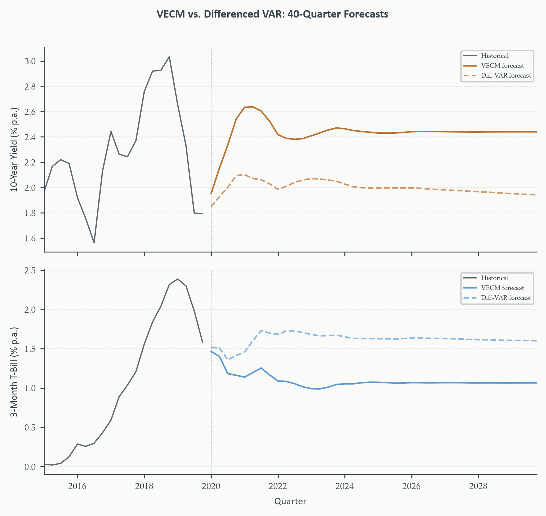
ignored: the differenced VAR implies a long-run term spread of 0.35 pp, less
than one quarter of the VECM's estimate of 1.37 pp.
jupyter: python3
format:
html:
toc: true
toc-depth: 3
toc-title: "In this chapter"
number-sections: true
code-fold: true
code-summary: "Show code"
code-tools: true
theme: cosmo
css: styles.css
highlight-style: github
fig-align: center
fig-cap-location: bottom
fig-responsive: true
html-math-method: mathjax
embed-resources: false
execute:
echo: true
warning: false
message: false
cache: false
---
```{python}
#| label: setup
#| include: false
import numpy as np
import pandas as pd
import matplotlib.pyplot as plt
import matplotlib as mpl
import matplotlib.ticker as mticker
from statsmodels.tsa.api import VAR
from statsmodels.tsa.vector_ar.vecm import VECM, coint_johansen
from statsmodels.tsa.stattools import adfuller, kpss, acf
from statsmodels.graphics.tsaplots import plot_acf, plot_pacf
import pandas_datareader.data as web
from datetime import datetime
import warnings
warnings.filterwarnings("ignore")
# ── EO Brand Palette ───────────────────────────────────────────────────────────
EO_CHARCOAL = "#36454F"
EO_COPPER = "#B87333"
EO_SAGE = "#87A96B"
EO_SKYBLUE = "#5B9BD5"
EO_TERRACOTTA = "#D4745E"
EO_LAVENDER = "#8E7AB5"
EO_COLORS = [EO_COPPER, EO_SKYBLUE, EO_SAGE,
EO_TERRACOTTA, EO_LAVENDER, EO_CHARCOAL]
PAGE_BG = "#FAFAF8"
# ── Global rcParams ────────────────────────────────────────────────────────────
mpl.rcParams.update({
"figure.figsize": (6, 3),
"figure.dpi": 150,
"figure.facecolor": PAGE_BG,
"figure.edgecolor": PAGE_BG,
"axes.facecolor": PAGE_BG,
"axes.edgecolor": EO_CHARCOAL,
"axes.linewidth": 0.7,
"axes.grid": True,
"axes.grid.axis": "y",
"axes.spines.top": False,
"axes.spines.right": False,
"axes.titlesize": 9,
"axes.titleweight": "bold",
"axes.titlecolor": EO_CHARCOAL,
"axes.titlelocation": "left",
"axes.labelsize": 8,
"axes.labelcolor": EO_CHARCOAL,
"axes.labelweight": "normal",
"axes.prop_cycle": mpl.cycler(color=EO_COLORS),
"grid.color": "#E5E5E5",
"grid.linewidth": 0.5,
"grid.linestyle": "--",
"grid.alpha": 0.8,
"xtick.color": EO_CHARCOAL,
"ytick.color": EO_CHARCOAL,
"xtick.labelsize": 7,
"ytick.labelsize": 7,
"xtick.direction": "out",
"ytick.direction": "out",
"xtick.major.size": 3,
"ytick.major.size": 3,
"lines.linewidth": 1.2,
"lines.solid_capstyle": "round",
"legend.frameon": True,
"legend.framealpha": 0.9,
"legend.edgecolor": "#CCCCCC",
"legend.facecolor": PAGE_BG,
"legend.fontsize": 6,
"legend.title_fontsize": 6,
"font.family": "serif",
"font.serif": ["Palatino Linotype", "Palatino", "Georgia",
"DejaVu Serif"],
"font.sans-serif": ["Calibri", "Arial", "DejaVu Sans"],
"font.size": 8,
"text.color": EO_CHARCOAL,
"savefig.dpi": 300,
"savefig.bbox": "tight",
"savefig.facecolor": PAGE_BG,
})
def eo_suptitle(fig, title, **kwargs):
defaults = dict(fontsize=9, fontweight="bold",
color=EO_CHARCOAL, fontfamily="Calibri", y=1.01)
defaults.update(kwargs)
fig.suptitle(title, **defaults)
def eo_style_ax(ax):
for obj in [ax.title, ax.xaxis.label, ax.yaxis.label]:
obj.set_fontfamily("Calibri")
RECESSIONS = [
("1960-04-01", "1961-02-01"),
("1969-12-01", "1970-11-01"),
("1973-11-01", "1975-03-01"),
("1980-01-01", "1980-07-01"),
("1981-07-01", "1982-11-01"),
("1990-07-01", "1991-03-01"),
("2001-03-01", "2001-11-01"),
("2007-12-01", "2009-06-01"),
]
def shade_recessions(ax, start=None, end=None):
for rec_start, rec_end in RECESSIONS:
s, e = pd.Timestamp(rec_start), pd.Timestamp(rec_end)
if start is not None and e < pd.Timestamp(start):
continue
if end is not None and s > pd.Timestamp(end):
continue
ax.axvspan(s, e, color=EO_CHARCOAL, alpha=0.08, lw=0)
def shade_inversions(ax, spread, index, start=None, end=None):
"""Shade periods when the yield spread is negative (curve inverted)."""
in_inv = False
inv_start = None
for i, (dt, val) in enumerate(zip(index, spread)):
if start is not None and dt < pd.Timestamp(start):
continue
if end is not None and dt > pd.Timestamp(end):
continue
if val < 0 and not in_inv:
inv_start = dt
in_inv = True
elif val >= 0 and in_inv:
ax.axvspan(inv_start, dt, color=EO_TERRACOTTA, alpha=0.18, lw=0)
in_inv = False
if in_inv:
ax.axvspan(inv_start, index[-1], color=EO_TERRACOTTA, alpha=0.18, lw=0)
```
```{python}
#| label: data-download
#| include: false
#| cache: true
from pathlib import Path
DATA_PATH = Path("../../data/raw")
start = datetime(1954, 1, 1)
end = datetime(2019, 12, 31) # pre-COVID sample throughout
# ── 10-year Treasury constant maturity yield (GS10, monthly) ──────────────────
gs10_raw = pd.read_csv(DATA_PATH / "GS10.csv", index_col="date", parse_dates=True).loc[str(start):str(end)]
gs10_raw.columns = ["GS10"]
# ── 3-month Treasury bill rate (TB3MS, monthly) ───────────────────────────────
tb3_raw = pd.read_csv(DATA_PATH / "TB3MS.csv", index_col="date", parse_dates=True).loc[str(start):str(end)]
tb3_raw.columns = ["TB3MS"]
# ── Resample to quarterly averages and merge ───────────────────────────────────
gs10_q = gs10_raw.resample("QS").mean()
tb3_q = tb3_raw.resample("QS").mean()
yields = gs10_q.join(tb3_q, how="inner").dropna()
yields.columns = ["LongRate", "ShortRate"]
yields["Spread"] = yields["LongRate"] - yields["ShortRate"]
yields = yields.loc["1954-01-01":"2019-10-01"].copy()
SAMPLE_START = yields.index[0].strftime("%Y-%m-%d")
SAMPLE_END = yields.index[-1].strftime("%Y-%m-%d")
# Data matrix for VAR / VECM estimation
yield_data = yields[["LongRate", "ShortRate"]]
```
::: {.callout-note}
## Learning Objectives
By the end of this chapter, you will be able to:
- Explain why a VAR in levels with I(1) variables produces unreliable inference,
and why differencing alone is not always the right remedy
- Define cointegration precisely: what a shared stochastic trend is, what the
cointegrating vector represents, and what cointegrating rank measures
- Apply the Johansen trace test step by step: construct the $\Pi$ matrix,
interpret its eigenvalues, compute the trace statistic, and determine rank
against critical value tables
- Articulate the role of deterministic components — intercepts and trends — in
the cointegrating space, and select the correct specification in practice
- Reparameterise a VAR in levels as a VECM, and interpret the $\alpha$ and
$\beta$ matrices as speed of adjustment and the long-run equilibrium vector
- Estimate a VECM on real data, read the error correction term economically,
and run standard residual diagnostics
- Produce impulse response functions from a VECM and interpret permanent and
transitory components of shocks
- Compare VECM and differenced-VAR forecasts and explain what cointegration
adds at long horizons
:::
This chapter takes up the question that Chapter 7 left open. We built the full
VAR toolkit there — lag selection, Granger causality, structural identification,
impulse responses — but maintained throughout that every variable in the system
is stationary. Section 7.9 showed what happens when that assumption fails: the
standard inference tools break down, and the two naive responses — estimating
the VAR in levels anyway, or differencing everything before estimation — are
both wrong in different ways. The cointegration framework is the principled
resolution. Section 8.1 makes the problem precise and introduces the yield
curve as the running example, showing why neither a levels VAR nor a differenced
VAR captures the full picture. Section 8.2 develops the concept of cointegration
itself: what a shared stochastic trend means, how it is formalised through the
cointegrating vector, and how the expectations hypothesis of the term structure
motivates the specific long-run restriction we impose. Section 8.3 develops the
Johansen procedure for testing cointegrating rank. Section 8.4 builds the VECM,
shows how it separates short-run dynamics from the long-run equilibrium, and
estimates it on our running example. Section 8.5 covers diagnostics and the
comparison between VECM and differenced-VAR residuals. Section 8.6 closes the
chapter with impulse responses and forecasts.
## The Problem with I(1) Variables in a VAR {#sec-problem}
Chapter 4 established that regressing one I(1) series on another produces
spurious results unless the two series are cointegrated: $t$-statistics are
inflated, $R^2$ is high even when the series are independent, and the residuals
exhibit strong serial correlation that invalidates standard inference. The same
problem — and a related but distinct set of problems — arises in a multivariate
setting when I(1) variables are included in a VAR estimated in levels.
The immediate concern is inference. The OLS coefficient estimates in each VAR
equation are still consistent when the variables are I(1) — unlike in a static
regression, the dynamics of the VAR prevent the worst forms of spurious
correlation — but the sampling distributions of those estimates are non-standard.
The $t$-statistics, $F$-statistics, and information criteria we used throughout
Chapter 7 for lag selection and Granger causality tests no longer have their
usual asymptotic distributions under the null. Lag selection by AIC or BIC
systematically over-selects. The block exclusion tests for Granger causality
reject too often even when there is no true predictive relationship. The
companion matrix may have eigenvalues close to the unit circle — not because
the system is explosive, but because the unit roots in the data are being
absorbed into the VAR dynamics.
The subtler problem emerges in forecasting and impulse response analysis. A
correctly specified stationary VAR has the property that shocks are transitory:
impulse responses decay to zero as the horizon grows, and long-run forecasts
revert to the unconditional mean. An I(1) system has no unconditional mean to
revert to. Shocks to an integrated variable are permanent — they shift the
level of the series indefinitely. A VAR in levels estimated on I(1) variables
will produce impulse responses that do not converge to zero, reflecting the
permanent effects of shocks. Depending on whether the variables are cointegrated
or not, those permanent effects either make economic sense or represent
a modelling artefact.
::: {.callout-warning icon=false}
## Do Not Estimate a VAR in Levels with I(1) Variables
If unit root tests indicate that one or more variables in your system are I(1),
a VAR estimated in levels produces non-standard inference for lag selection,
Granger causality, and impulse responses. The correct path is:
1. Test each variable for unit roots (ADF and KPSS, as in Chapter 4).
2. If the variables are I(1), test for cointegration (Johansen procedure,
Section 8.3).
3. If cointegration is found, estimate a VECM (Section 8.4).
4. If no cointegration is found, estimate a VAR in first differences.
A VAR in levels with I(1) variables is neither option 3 nor option 4.
:::
### Differencing Restores Stationarity but Discards Long-Run Information
The obvious remedy is to difference the I(1) variables before including them
in the VAR. If $y_t \sim I(1)$, then $\Delta y_t \sim I(0)$, and a VAR
estimated on the differenced series is stationary. All the tools of Chapter 7
apply. The estimated coefficients have standard asymptotic distributions.
Granger causality tests are valid. Impulse responses decay to zero.
So what is the problem? The problem is that differencing discards information
about the levels of the variables — specifically, information about the long-run
relationships between them. If two I(1) series tend to move together over time —
if they share a common stochastic trend — then their levels are bound together
in a way that their differences cannot capture. A VAR in differences treats the
two series as if they drift independently, and it will produce forecasts that
diverge over long horizons even when the data tell us clearly that the series
belong together.
This is not a subtle econometric point. It has immediate economic content. If
the long rate and the short rate are both driven by the same monetary policy
and inflation expectations — if there is a stable long-run relationship between
them — then a model of $\Delta r^{10}_t$ and $\Delta r^{3m}_t$ cannot represent
that relationship. It can describe how changes in the two rates comove, but it
has no mechanism for pulling them back toward their long-run spread when they
drift apart. The error correction term — the variable that does that pulling —
is invisible to the differenced VAR.
::: {.callout-note}
## What "Long-Run Information" Means
The phrase "long-run information" has a precise meaning in this context. When
two I(1) series are cointegrated, there exists a linear combination of their
levels that is stationary — a combination that fluctuates around a stable mean.
That linear combination encodes the equilibrium relationship between the two
variables. A VAR in differences cannot estimate that relationship because it
never sees the levels; it only sees the period-to-period changes. The VECM
restores access to the levels relationship by including the lagged equilibrium
residual — the error correction term — as an additional regressor in each
equation. The VAR in differences omits that term entirely.
:::
### The Yield Curve: A Canonical Cointegration Example
We now ground the abstract discussion in the pair of series that serves as the
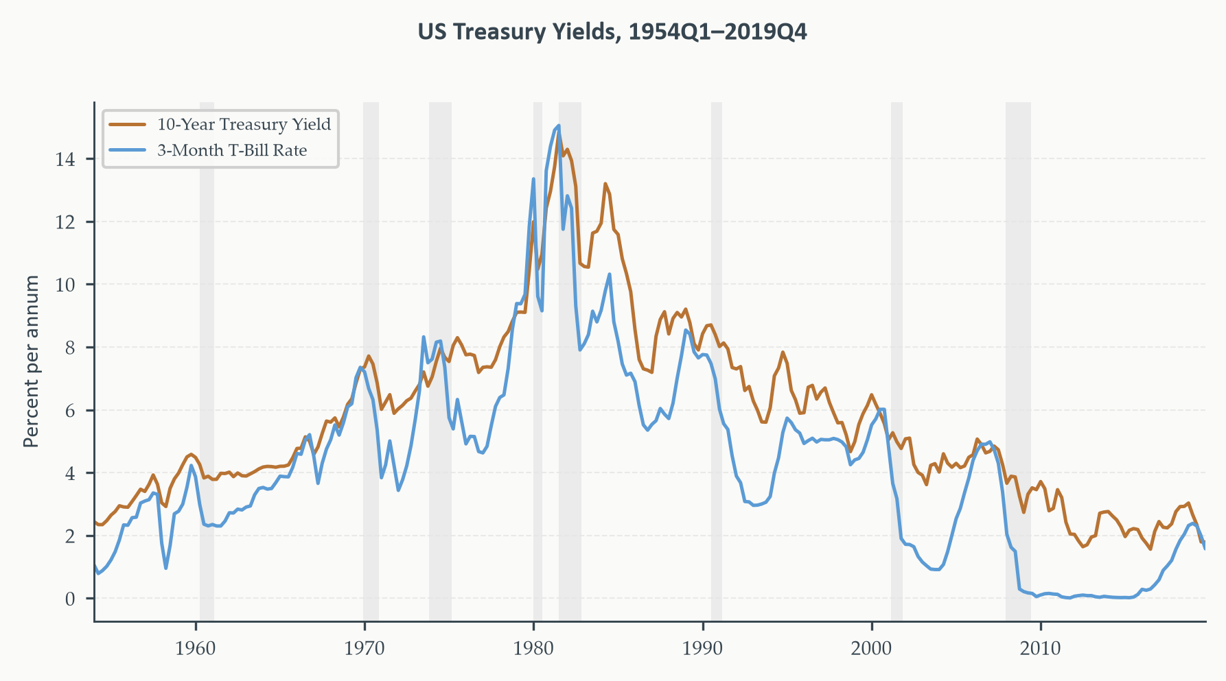
running example for this chapter. Figure 8.1 plots the 10-year Treasury constant
maturity yield and the 3-month Treasury bill rate for the United States from
1954Q1 through 2019Q4, constructed from FRED series [`GS10`](https://fred.stlouisfed.org/series/GS10) and [`TB3MS`](https://fred.stlouisfed.org/series/TB3MS), resampled
to quarterly averages. We restrict to the pre-COVID sample for the same reasons
given in previous chapters.
Both rates are I(1) over most samples — they wander without reverting to a fixed
level, driven by slowly shifting inflation expectations and the monetary policy
stance. Yet they move together with a consistency that goes beyond coincidence.
Both rates rose through the 1970s as inflation climbed, peaked in the early
1980s with the Volcker disinflation, and trended downward through the subsequent
decades as inflation and its expectations fell. Whatever drives one rate at low
frequencies drives both. This is the hallmark of a shared stochastic trend.
```{python}
#| label: fig-yields
#| fig-cap: "The 10-year Treasury yield (copper) and the 3-month Treasury bill
#| rate (sky blue), 1954Q1–2019Q4. Both rates are I(1): they drift upward
#| through the inflationary 1970s and downward through the post-Volcker
#| decades without reverting to a fixed level. Yet they track each other
#| closely throughout — driven by the same monetary policy and inflation
#| expectations — motivating the hypothesis that they share a common
#| stochastic trend. Recessions shaded in grey."
fig, ax = plt.subplots(figsize=(6, 3.2))

ax.plot(yields.index, yields["LongRate"],
        color=EO_COPPER, lw=1.2, label="10-Year Treasury Yield")
ax.plot(yields.index, yields["ShortRate"],
        color=EO_SKYBLUE, lw=1.2, label="3-Month T-Bill Rate")

shade_recessions(ax, start=SAMPLE_START, end=SAMPLE_END)
ax.set_xlim(yields.index[0], yields.index[-1])
ax.set_ylabel("Percent per annum")
ax.legend(loc="upper left", fontsize=6)
eo_style_ax(ax)
eo_suptitle(fig, "US Treasury Yields, 1954Q1–2019Q4")
fig.tight_layout()
plt.show()
```
*The 10-year yield (copper) and the 3-month T-bill rate (sky blue). Both series
are clearly non-stationary in levels, trending upward through the inflationary
1970s and declining after the Volcker disinflation. They track each other
throughout the sample, moving in the same direction over long horizons even
though their gap — the term spread — fluctuates considerably in the short run.*
Formal unit root tests confirm the visual impression.
```{python}
#| label: tbl-unit-root-yields
#| code-summary: "Show code"
print(f"{'─'*60}")
print(f"  Unit Root Tests — 10-Year Yield and 3-Month T-Bill")
print(f"  Intercept included; no deterministic trend.")
print(f"{'─'*60}")
print(f"  ADF  H₀: series has a unit root  (reject → stationary)")
print(f"  KPSS H₀: series is stationary    (reject → unit root) ")
print(f"{'─'*60}")

for name, col in [("10-Year Yield", "LongRate"), ("3-Month T-Bill", "ShortRate")]:
    y = yields[col].dropna()
    adf_stat, adf_p, _, _, adf_cv, _ = adfuller(y, autolag="AIC", regression="c")
    kpss_stat, kpss_p, _, kpss_cv = kpss(y, regression="c", nlags="auto")
    adf_dec  = "Fail to reject" if adf_p  > 0.05 else "Reject"
    kpss_dec = "Reject" if kpss_stat > kpss_cv["5%"] else "Fail to reject"
    print(f"\n  {name}")
    print(f"  {'─'*52}")
    print(f"  ADF statistic  : {adf_stat:>8.3f}   p-value: {adf_p:.3f}   {adf_dec}")
    print(f"  ADF 5% c.v.    : {adf_cv['5%']:>8.3f}")
    print(f"  KPSS statistic : {kpss_stat:>8.3f}   p-value: {kpss_p:.3f}   {kpss_dec}")
    print(f"  KPSS 5% c.v.   : {kpss_cv['5%']:>8.3f}")

print(f"\n{'─'*60}")
print(f"  Both series: ADF fails to reject unit root;")
print(f"  KPSS rejects stationarity. Confirmed I(1).")
print(f"{'─'*60}")
```
*Unit root tests for the 10-year Treasury yield and the 3-month T-bill rate,
1954Q1–2019Q4. An intercept but no deterministic trend is included, since
interest rates do not trend in one direction indefinitely. The ADF fails to
reject the unit root null for both series (p-values of 0.74 and 0.58); the
KPSS rejects the null of stationarity for both (statistics of 0.65 and 0.72,
both exceeding the 5% critical value of 0.46). The tests agree: both rates
are I(1).*
Now consider the spread — the difference between the 10-year yield and the
3-month rate. The expectations hypothesis of the term structure predicts that
this spread is stationary: both rates share the same long-run level of short
rates (averaged over expectations), so their difference should fluctuate around
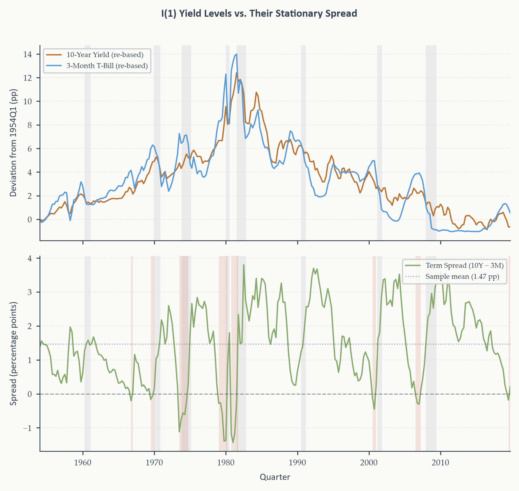
a constant term premium rather than drifting. Figure 8.2 shows the spread
alongside the two individual rates, and the contrast is immediate.
```{python}
#| label: fig-spread
#| fig-cap: "The 10-year/3-month term spread (bottom panel) alongside the two
#| yield levels re-based to 1954Q1 (top panel). The individual rates drift
#| without bound; the spread fluctuates around a positive mean and shows no
#| long-run drift. Terracotta shading marks yield curve inversions — periods
#| when the spread turns negative — which have preceded every recession in the
#| sample. Grey shading marks NBER recessions."
fig, axes = plt.subplots(2, 1, figsize=(6, 5.5), sharex=True)

# Top panel: levels re-based to zero
axes[0].plot(yields.index,
             yields["LongRate"] - yields["LongRate"].iloc[0],
             color=EO_COPPER, lw=1.1, label="10-Year Yield (re-based)")
axes[0].plot(yields.index,
             yields["ShortRate"] - yields["ShortRate"].iloc[0],
             color=EO_SKYBLUE, lw=1.1, label="3-Month T-Bill (re-based)")
axes[0].set_ylabel("Deviation from 1954Q1 (pp)")
axes[0].legend(fontsize=6, loc="upper left")
shade_recessions(axes[0], start=SAMPLE_START, end=SAMPLE_END)
axes[0].set_xlim(yields.index[0], yields.index[-1])
eo_style_ax(axes[0])

# Bottom panel: spread with inversion shading
axes[1].plot(yields.index, yields["Spread"], color=EO_SAGE, lw=1.1,
             label="Term Spread (10Y − 3M)")
axes[1].axhline(0, color=EO_CHARCOAL, lw=0.8, ls="--", alpha=0.5)
axes[1].axhline(yields["Spread"].mean(), color=EO_CHARCOAL, lw=0.8,
                ls=":", alpha=0.5,
                label=f"Sample mean ({yields['Spread'].mean():.2f} pp)")
shade_inversions(axes[1], yields["Spread"].values, yields.index,
                 start=SAMPLE_START, end=SAMPLE_END)
shade_recessions(axes[1], start=SAMPLE_START, end=SAMPLE_END)
axes[1].set_ylabel("Spread (percentage points)")
axes[1].set_xlabel("Quarter")
axes[1].legend(fontsize=6, loc="upper right")
axes[1].set_xlim(yields.index[0], yields.index[-1])
eo_style_ax(axes[1])

eo_suptitle(fig, "I(1) Yield Levels vs. Their Stationary Spread")
fig.tight_layout()
plt.show()
```
*Top panel: the 10-year yield and the 3-month T-bill rate re-based to their
1954Q1 values, illustrating the non-stationary drift common to both. Bottom
panel: the term spread, which fluctuates around a positive mean throughout the
sample without any long-run drift — the cointegration signature. Terracotta
shading marks yield curve inversions; grey shading marks NBER recessions.
Every recession in the sample was preceded by an inversion.*
The spread panel tells the story cleanly. Unlike the individual rates, which
share the stochastic trend of the monetary cycle, the spread is visibly
mean-reverting: it widens, narrows, occasionally turns negative, and pulls
back toward its long-run average. This is exactly what cointegration predicts —
the common stochastic trend cancels when the spread is formed, leaving a
stationary residual. Crucially, the figure also highlights the **[yield curve
inversion](https://en.wikipedia.org/wiki/Inverted_yield_curve)** — the period when the spread crosses zero from above, shaded in
terracotta. In the [VECM](https://en.wikipedia.org/wiki/Error_correction_model#VECM) framework, an inversion means the error correction
term has turned negative: the system is below its long-run equilibrium, and
the adjustment mechanism implies forces that push the spread back up. The
near-perfect record of inversions preceding recessions — visible in the
alignment of terracotta and grey shading — is one of the most robust empirical
regularities in macroeconomics, and the VECM gives a natural language for
understanding it: inversions are extreme deviations from the long-run
equilibrium of the yield curve, and the subsequent correction drives both
short and long rates.
A natural question is why we use the Treasury yield pair rather than other
well-known I(1) pairs in macroeconomics. The short answer is clarity. Some
pairs that are theoretically cointegrated — log consumption and log income, for
instance, as implied by the permanent income hypothesis — turn out to have
equilibrium relationships that shift substantially over long samples. The US
personal saving rate has trended downward since the 1970s, meaning the
consumption-to-income ratio is not cleanly stationary over a postwar sample.
A Chow test or Bai-Perron procedure of the kind developed in Chapter 6 would
detect a structural break in that long-run relationship. The yield curve does
not suffer from this problem: the term spread has fluctuated around a positive
mean for the full postwar period without any comparable secular drift, making
it the cleaner illustration of cointegration mechanics.
## Cointegration: The Concept {#sec-cointegration}
### A Shared Stochastic Trend
How can two non-stationary series produce a stationary combination? The answer
lies in the structure of integrated processes. Recall from Chapter 4 that a
random walk $y_t = y_{t-1} + \varepsilon_t$ accumulates its shocks: we can
write $y_t = y_0 + \sum_{s=1}^{t} \varepsilon_s$, where the partial sum
$\sum_{s=1}^{t} \varepsilon_s$ grows without bound as $t$ increases. This
accumulated sum is the stochastic trend in $y_t$ — it is what makes the series
non-stationary.
Now suppose two series, $y_t$ and $x_t$, accumulate the *same* stochastic
trend. Write:
$$\begin{aligned}
y_t &= \mu_y + \tau_t + u_t^y \\
x_t &= \mu_x + \tau_t + u_t^x
\end{aligned}$$
where $\tau_t = \tau_{t-1} + \eta_t$ is the common stochastic trend — a random
walk driven by shocks $\eta_t$ — and $u_t^y$, $u_t^x$ are stationary
disturbances. Each series individually is I(1), because the common trend $\tau_t$
is non-stationary and it enters both equations. But now form the difference:
$$y_t - x_t = (\mu_y - \mu_x) + (u_t^y - u_t^x)$$
The common trend $\tau_t$ cancels exactly. What remains is a constant plus the
difference of two stationary processes — and that difference is itself
stationary. Two I(1) series can therefore produce a stationary linear
combination precisely when they share a common stochastic trend that cancels
when the combination is formed.
This is the essence of [cointegration](https://en.wikipedia.org/wiki/Cointegration): the non-stationarity in both series comes
from the same source, so it can be subtracted away. Cointegrated series are
sometimes described as moving together in the long run — not in the sense that
they are always equal or always close, but in the sense that their deviations
from each other are bounded. Shocks may push them apart temporarily, but an
equilibrating force eventually pulls them back.
::: {.callout-note}
## Definition 8.1 — Cointegration
Two I(1) series $y_t$ and $x_t$ are **cointegrated** if there exists a constant
$\beta$ such that
$$z_t = y_t - \beta x_t$$
is I(0). The vector $(1, -\beta)'$ is called the **cointegrating vector**, and
$z_t$ is the **equilibrium residual** or **error correction term**. The
cointegrating vector is not unique without a normalisation: if $(1, -\beta)'$
is a cointegrating vector, then $(c, -c\beta)'$ is also one for any $c \neq 0$.
We normalise by setting the coefficient on $y_t$ to 1.
:::
The definition extends naturally to systems with more than two variables. If
$\mathbf{y}_t = (y_{1t}, y_{2t}, \ldots, y_{nt})'$ is a vector of I(1) series,
a cointegrating vector is any $n \times 1$ vector $\boldsymbol{\beta}$ such that
$\boldsymbol{\beta}' \mathbf{y}_t$ is I(0). The number of linearly independent
cointegrating vectors is the **cointegrating rank**, which we discuss in
Section 8.2.4.
### The Cointegrating Vector and the Equilibrium Residual
The cointegrating vector $\boldsymbol{\beta}$ has a direct economic
interpretation: it describes the long-run proportional relationship between the
variables. To see this, suppose $z_t = y_t - \beta x_t$ is stationary with
mean $\mu_z$. Then in the long run, when $z_t$ is at its mean, we have:
$$y_t = \mu_z + \beta x_t \tag{8.1}$$
This is a long-run equilibrium relationship. The coefficient $\beta$ gives the
long-run response of $y_t$ to a permanent change in $x_t$. The equilibrium
residual $z_t = y_t - \beta x_t - \mu_z$ measures the current deviation from
that long-run relationship. When $z_t > 0$, $y_t$ is above its long-run
equilibrium value given $x_t$; when $z_t < 0$, it is below.
The equilibrium residual is stationary by definition — it fluctuates around
zero, occasionally deviating but always returning. This stationarity is what
makes the long-run relationship meaningful. If $z_t$ were non-stationary, the
deviation from equilibrium would grow without bound, and there would be no
meaningful sense in which the two variables are related in the long run.
For the 10-year yield ($y_t = r^{10}_t$) and the 3-month rate ($x_t = r^{3m}_t$),
the cointegrating vector gives the long-run response of the long rate to the
short rate. If $\beta = 1$, then the long-run relationship is
$r^{10}_t = \mu_z + r^{3m}_t$, meaning the two rates move one-for-one in the
long run and their spread $r^{10}_t - r^{3m}_t$ is stationary around a constant
term premium $\mu_z$. This is precisely what the expectations hypothesis
predicts, and it is exactly the picture in the bottom panel of Figure 8.2.
The yield curve inversion corresponds to a period when the equilibrium residual
$z_t$ turns negative — the spread has fallen below its long-run mean — and the
VECM's adjustment mechanism predicts a subsequent correction back toward
positive territory.
### The Expectations Hypothesis as an Identifying Restriction
The [expectations hypothesis](https://en.wikipedia.org/wiki/Expectations_hypothesis) of the term structure (EH) is one of the oldest
and most tested relationships in financial economics. Its logic is simple: if
financial markets are efficient and investors care only about expected returns,
then the yield on a long-term bond must equal the average of expected future
short-term rates plus a constant risk premium. A 10-year bond should yield
roughly what an investor expects to earn by rolling over 3-month T-bills for
ten years, adjusted for the compensation required for bearing interest rate risk.
The long-run implication for cointegration is direct. Both the long rate and
the short rate are driven by the same underlying monetary policy and inflation
expectations — the same stochastic trend. In the short run, the spread between
them fluctuates as expectations shift and risk appetite varies. But in the long
run, neither rate can drift permanently away from the other: if the long rate
were permanently above the short rate by an ever-widening margin, arbitrage
would close the gap. The spread is therefore bounded — stationary — and the
two rates are cointegrated with the cointegrating vector $(1, -1)'$ implied by
the EH restriction $\beta = 1$.
This restriction is testable. We can estimate $\beta$ freely from the data and
ask whether the estimate is statistically indistinguishable from one. If the
data support $\beta = 1$, the simple EH is consistent with the evidence. If
$\beta$ differs from one, something more complicated is at work — perhaps a
time-varying term premium, or a structural break in the relationship during
the zero-lower-bound period after 2008. We make no prior commitment to the
outcome. The Johansen procedure estimates $\beta$ as part of the cointegration
analysis, and we will report what the data say.
::: {.callout-warning icon=false}
## Cointegration Does Not Imply Causality
The cointegrating vector tells us the long-run proportional relationship between
two variables, not which one causes the other. If $r^{10}_t$ and $r^{3m}_t$ are
cointegrated with vector $(1, -\beta)'$, the equilibrium residual $z_t =
r^{10}_t - \beta r^{3m}_t$ is stationary. But this does not tell us whether
the long rate adjusts to the short rate, the short rate adjusts to the long
rate, or both adjust. The Federal Reserve directly controls short rates and
influences long rates through expectations — so in a causal sense the short
rate drives the long. But the VECM may find that long rates also predict
short-rate changes, because the spread contains information about future Fed
policy. The $\alpha$ coefficients in the VECM — estimated in Section 8.4 —
answer the adjustment question empirically.
:::
### Cointegrating Rank: From Pairs to Systems
When we have more than two I(1) variables, there may be more than one
independent long-run relationship. A system of $n$ I(1) variables can have
at most $n - 1$ linearly independent cointegrating vectors — if there were $n$,
the system would be stationary, contradicting the assumption that the variables
are I(1).
The **cointegrating rank** $r$ is the number of linearly independent
cointegrating vectors. It can range from $0$ to $n - 1$:
- $r = 0$: no cointegration. The variables share no common stochastic trends,
and a VAR in first differences is the correct model. The system has $n$
independent stochastic trends.
- $0 < r < n$: partial cointegration. There are $r$ long-run equilibrium
relationships and $n - r$ independent stochastic trends driving the system.
The VECM is the correct model.
- $r = n - 1$: the system has a single common stochastic trend. There are
$n - 1$ cointegrating relationships tying all variables together.
- $r = n$: impossible for I(1) variables. This would imply the variables are
stationary.
For our two-variable system of the 10-year yield and the 3-month rate, the
possible ranks are $r = 0$ (no cointegration, each rate has its own independent
stochastic trend) and $r = 1$ (one cointegrating relationship, one common
stochastic trend). The expectations hypothesis predicts $r = 1$. We will verify
this formally using the Johansen trace test in Section 8.3.
The connection between cointegrating rank and common trends is worth dwelling
on. With $r = 1$ in a two-variable system, one cointegrating vector removes
one stochastic trend, leaving a single common trend that drives both series.
That common trend is the monetary policy and inflation expectations trend that
both rates share. The cointegrating vector — the term spread — is the linear
combination that eliminates it.
::: {.callout-note}
## The Common Trends Representation
A system of $n$ I(1) variables with cointegrating rank $r$ can be written as:
$$\mathbf{y}_t = \boldsymbol{\Gamma} \mathbf{f}_t + \boldsymbol{\xi}_t \tag{8.2}$$
where $\mathbf{f}_t$ is a $(n - r) \times 1$ vector of **common stochastic
trends** (random walks), $\boldsymbol{\Gamma}$ is an $n \times (n - r)$ loading
matrix, and $\boldsymbol{\xi}_t$ is a vector of stationary disturbances. Each
variable in $\mathbf{y}_t$ is a linear combination of the $n - r$ common trends
plus a transitory component. Cointegration means the variables share fewer
independent trends than there are variables — the $n - r$ trends are the
"common" part, and the $r$ cointegrating vectors are exactly the linear
combinations that eliminate all $n - r$ trends simultaneously.
Equation (8.2) is called the **Stock-Watson common trends representation**, after
the influential 1988 paper by James Stock and Mark Watson that formalised this
decomposition.
:::
The rank determination problem — how many cointegrating vectors does a given
system actually have? — is the central question of Section 8.3. The Johansen
procedure answers it by examining the rank of a particular matrix derived from
the VAR in levels. For the yield curve, we expect the answer to be $r = 1$:
one shared trend (the monetary policy cycle), one cointegrating vector (the
term spread). The test should confirm this — and if it does not, we have learned
something economically interesting about the independence of long and short
rates that demands explanation.
We now develop the test.
## Testing for Cointegration: The Johansen Procedure {#sec-johansen}
### From VAR to the $\Pi$ Matrix
The [Johansen procedure](https://en.wikipedia.org/wiki/Johansen_test) begins not with a new model but with the VAR in levels
we were warned against estimating for inference — because despite its inferential
problems, the levels VAR contains the information needed to test for
cointegration. The key insight is that cointegrating relationships, if they
exist, impose a specific algebraic restriction on the VAR coefficient matrices:
the matrix that collects the long-run information has reduced rank. Testing for
cointegration is therefore a test of the rank of a particular matrix, and rank
can be determined from eigenvalues.
Start with a VAR($p$) in levels for an $n \times 1$ vector of I(1) variables
$\mathbf{y}_t$:
$$\mathbf{y}_t = \mathbf{c} + \mathbf{A}_1 \mathbf{y}_{t-1} +
\mathbf{A}_2 \mathbf{y}_{t-2} + \cdots +
\mathbf{A}_p \mathbf{y}_{t-p} + \mathbf{u}_t \tag{8.3}$$
Subtract $\mathbf{y}_{t-1}$ from both sides and collect terms. After some
rearrangement — the same algebra used to convert an AR($p$) into an ADF
regression in Chapter 4 — the VAR in levels can be written as:
$$\Delta \mathbf{y}_t = \mathbf{c} + \boldsymbol{\Pi} \mathbf{y}_{t-1} +
\boldsymbol{\Gamma}_1 \Delta\mathbf{y}_{t-1} + \cdots +
\boldsymbol{\Gamma}_{p-1} \Delta\mathbf{y}_{t-p+1} + \mathbf{u}_t \tag{8.4}$$
where the matrices $\boldsymbol{\Gamma}_i$ collect the short-run dynamics and
the matrix $\boldsymbol{\Pi}$ collects the long-run information:
$$\boldsymbol{\Pi} = \sum_{i=1}^{p} \mathbf{A}_i - \mathbf{I}_n, \qquad
\boldsymbol{\Gamma}_i = -\sum_{j=i+1}^{p} \mathbf{A}_j$$
Equation (8.4) is called the **vector error correction representation** of the
VAR. It looks like a VAR in differences augmented by one extra term:
$\boldsymbol{\Pi} \mathbf{y}_{t-1}$, which involves the lagged *levels* of the
variables. This is the term that carries long-run information.
The rank of $\boldsymbol{\Pi}$ determines the cointegrating structure of the
system. To see why, consider what happens under different rank assumptions:
- **$\text{rank}(\boldsymbol{\Pi}) = 0$:** $\boldsymbol{\Pi} = \mathbf{0}$.
The lagged levels term vanishes entirely. Equation (8.4) becomes a VAR in
first differences — exactly the specification appropriate when there is no
cointegration. Each variable has its own independent stochastic trend.
- **$\text{rank}(\boldsymbol{\Pi}) = r$, with $0 < r < n$:** $\boldsymbol{\Pi}$
has reduced rank $r$. It can be written as the product of two $n \times r$
matrices of rank $r$:
$$\boldsymbol{\Pi} = \boldsymbol{\alpha} \boldsymbol{\beta}' \tag{8.5}$$
where $\boldsymbol{\beta}$ contains the $r$ cointegrating vectors as its
columns, and $\boldsymbol{\alpha}$ contains the speed-of-adjustment
coefficients. The term $\boldsymbol{\Pi} \mathbf{y}_{t-1} = \boldsymbol{\alpha}
\boldsymbol{\beta}' \mathbf{y}_{t-1}$ is then an $n \times 1$ vector of $r$
stationary error correction terms, each premultiplied by the adjustment
coefficients that determine how strongly each variable responds. This is the
VECM, which Section 8.4 develops in full.
- **$\text{rank}(\boldsymbol{\Pi}) = n$:** $\boldsymbol{\Pi}$ has full rank.
The variables are stationary in levels, contradicting the I(1) assumption.
This case is ruled out by design when we begin with confirmed I(1) variables.
::: {.callout-note}
## The $\Pi$ Matrix Is the Heart of the Johansen Test
Everything in the Johansen procedure flows from the rank of $\boldsymbol{\Pi}$.
The test does not directly examine the cointegrating vectors — it examines the
eigenvalues of a matrix derived from $\boldsymbol{\Pi}$. A zero eigenvalue
means $\boldsymbol{\Pi}$ is rank-deficient in that direction; $r$ non-zero
eigenvalues means $\text{rank}(\boldsymbol{\Pi}) = r$ and there are $r$
cointegrating relationships. Counting the non-zero eigenvalues is therefore
equivalent to determining the cointegrating rank.
:::
### Eigenvalues and the Rank of $\Pi$: A Numerical Walkthrough
Before turning to the formal test, it is worth building intuition about what
eigenvalues reveal about rank. Consider a concrete $2 \times 2$ example
calibrated to the yield curve — two I(1) variables, the 10-year yield ($y_{1t}$)
and the 3-month rate ($y_{2t}$) — and suppose the true $\boldsymbol{\Pi}$
matrix is:
$$\boldsymbol{\Pi} = \begin{bmatrix} -0.05 & 0.05 \\ 0.12 & -0.12 \end{bmatrix}$$
Notice that the second column is exactly $-1$ times the first. This matrix has
rank 1 — one of its eigenvalues must be zero, because the two columns are
linearly dependent. We can verify this directly: the eigenvalues of
$\boldsymbol{\Pi}$ are found from $\det(\boldsymbol{\Pi} - \lambda \mathbf{I}) = 0$:
$$\det \begin{bmatrix} -0.05 - \lambda & 0.05 \\ 0.12 & -0.12 - \lambda \end{bmatrix}
= (-0.05 - \lambda)(-0.12 - \lambda) - (0.05)(0.12) = 0$$
Expanding:
$$\lambda^2 + 0.17\lambda + 0.006 - 0.006 = \lambda^2 + 0.17\lambda = 0$$
So $\lambda(\lambda + 0.17) = 0$, giving eigenvalues $\lambda_1 = 0$ and
$\lambda_2 = -0.17$. One eigenvalue is exactly zero, confirming rank 1.
Now write $\boldsymbol{\Pi} = \boldsymbol{\alpha}\boldsymbol{\beta}'$ with
$r = 1$. We can read off:
$$\boldsymbol{\alpha} = \begin{bmatrix} -0.05 \\ 0.12 \end{bmatrix}, \qquad
\boldsymbol{\beta}' = \begin{bmatrix} 1 & -1 \end{bmatrix}$$
The cointegrating vector is $(1, -1)'$: the long-run relationship is
$y_{1t} - y_{2t} = \text{constant}$ — the 10-year yield minus the 3-month
rate equals a constant term premium. This is exactly the EH restriction
$\beta = 1$. The adjustment coefficients say that when the spread narrows
below its long-run mean (negative error correction term), the long rate rises
by 0.05 times the deviation and the short rate falls by 0.12 times the
deviation — both forces widening the spread and pushing the system back toward
equilibrium. The short rate adjusts more strongly than the long rate, which
is intuitive: the Fed controls short rates actively in response to economic
conditions, while long rates move more sluggishly.
In practice, we never observe $\boldsymbol{\Pi}$ — we estimate it from the
data, and the estimated eigenvalues are random variables. The Johansen test
uses the magnitudes of the sample eigenvalues to make inference about how many
population eigenvalues are non-zero.
### The Trace Statistic and Maximum Eigenvalue Statistic
The Johansen procedure estimates equation (8.4) by OLS and computes the
eigenvalues $\hat{\lambda}_1 \geq \hat{\lambda}_2 \geq \cdots \geq \hat{\lambda}_n$
of a particular matrix derived from the residuals. Under the null hypothesis
of rank $r$, the $n - r$ smallest eigenvalues should be close to zero; under
the alternative, they should be positive and bounded away from zero.
::: {.callout-note}
## How the Eigenvalues Are Computed
The eigenvalues in the Johansen procedure are not eigenvalues of $\hat{\boldsymbol{\Pi}}$
directly. They come from a **reduced-rank regression** that concentrates out
the short-run dynamics $\boldsymbol{\Gamma}_i \Delta\mathbf{y}_{t-i}$ first,
then finds the $r$ linear combinations of $\mathbf{y}_{t-1}$ that are most
correlated with $\Delta \mathbf{y}_t$ after that partialling out. The resulting
eigenvalues $\hat{\lambda}_i$ are squared canonical correlations between
$\Delta \mathbf{y}_t$ and $\mathbf{y}_{t-1}$, adjusted for short-run dynamics.
They lie in $[0, 1]$: an eigenvalue of zero means the corresponding linear
combination of $\mathbf{y}_{t-1}$ has no predictive content for $\Delta
\mathbf{y}_t$ — it is non-stationary; an eigenvalue close to 1 means it has
strong predictive content — it is stationary, i.e., a cointegrating combination.
:::
Two test statistics are constructed from the eigenvalues.
The **trace statistic** tests the null hypothesis that the cointegrating rank
is at most $r$ against the alternative that it is greater than $r$:
$$\lambda_{\text{trace}}(r) = -T \sum_{i=r+1}^{n} \ln(1 - \hat{\lambda}_i) \tag{8.6}$$
Intuitively, if the null $\text{rank} \leq r$ is true, the eigenvalues
$\hat{\lambda}_{r+1}, \ldots, \hat{\lambda}_n$ should all be near zero, making
$\ln(1 - \hat{\lambda}_i) \approx 0$ and the statistic small. If any of those
eigenvalues is substantially positive, the statistic grows, and we reject the
null in favour of higher rank.
The **maximum eigenvalue statistic** tests $\text{rank} = r$ against
$\text{rank} = r + 1$ specifically:
$$\lambda_{\max}(r, r+1) = -T \ln(1 - \hat{\lambda}_{r+1}) \tag{8.7}$$
It isolates the contribution of the single next eigenvalue, making it more
focused than the trace statistic but also less powerful when rank exceeds
$r + 1$.
In practice we use the trace statistic as the primary test, because it has better
power properties when the true rank exceeds the null by more than one. The
maximum eigenvalue statistic serves as a check.
### Critical Values and the Rank Decision Rule
The trace and maximum eigenvalue statistics do not have standard chi-squared
distributions under the null. They follow non-standard distributions that depend
on $n - r$ — the number of unit roots being tested — and on the deterministic
components included in the model. Critical values are tabulated; `statsmodels`
reports them automatically.
The sequential testing procedure works as follows. Start at the most restrictive
null, $r = 0$ (no cointegration), and test against the alternative $r \geq 1$.
If the trace statistic exceeds the critical value, reject the null and move to
$r = 1$. Test $r = 1$ against $r \geq 2$. Continue until the null is not
rejected. The rank at which we first fail to reject is the estimated
cointegrating rank $\hat{r}$.
::: {.callout-warning icon=false}
## Sequential Testing Inflates the Type I Error Rate
Testing $r = 0$, then $r = 1$, then $r = 2$, and so on involves multiple
hypothesis tests. Each test has its own probability of a Type I error, and the
sequential procedure does not control the overall error rate at the nominal level.
In practice, this means the Johansen procedure may slightly over-reject the null
of low rank. Two remedies are common: use the Bartlett small-sample correction
(available as an option in some implementations), or treat the test results as
strongly suggestive rather than definitive and check robustness by estimating
VECMs at adjacent ranks.
:::
### Deterministic Components in the Cointegrating Space
Before running the Johansen test, we must specify the deterministic components
in equation (8.4): whether to include an intercept, a trend, or both, and
whether those components enter the cointegrating relationship, the short-run
dynamics, or both. This choice matters — the wrong specification changes the
critical values and can alter the rank conclusion.
There are five standard cases, but two are relevant for most applications:
**Case 2 (restricted intercept, no trend):** The long-run relationship has a
non-zero mean — $\boldsymbol{\beta}'\mathbf{y}_t = \mu_0$ — but the variables
do not trend deterministically. Use this when the I(1) variables have no drift
and the cointegrating relationship has a non-zero intercept.
**Case 3 (unrestricted intercept, no deterministic trend in the cointegrating
space):** Both the cointegrating relationship and the short-run equations include
an intercept, allowing the levels of the variables to drift linearly. Use this
when the I(1) variables have drift — as interest rates clearly do over long
samples — but the cointegrating relationship itself does not trend.
For the yield curve, Case 2 is the natural starting point. Interest rates do
not trend in one direction indefinitely — the secular decline of the post-Volcker
period was a long but ultimately bounded episode. The EH implies the spread
fluctuates around a constant term premium with no deterministic trend. We
therefore use `det_order = 0` in `coint_johansen`, which corresponds to a
restricted constant in the cointegrating space.
::: {.callout-warning icon=false}
## The `det_order` Argument in `coint_johansen`
In `statsmodels`, the `coint_johansen` function's `det_order` argument controls
the deterministic specification:
- `det_order = -1`: no deterministic terms
- `det_order = 0`: restricted intercept in the cointegrating space (Case 2)
- `det_order = 1`: unrestricted intercept, allowing a linear trend in levels
(Case 3)
For the yield curve with no secular trend in the spread, use `det_order = 0`.
For trended I(1) series where the levels themselves trend, use `det_order = 1`.
Using the wrong `det_order` applies incorrect critical values and can change
the rank conclusion.
:::
### Empirical Application: The US Yield Curve
We now apply the Johansen procedure to the 10-year yield and the 3-month
T-bill rate over the 1954Q1–2019Q4 sample. The first step is lag length
selection for the underlying VAR in levels.
```{python}
#| label: tbl-var-lag-selection
#| code-summary: "Show code"
print(f"{'─'*60}")
print(f"  VAR Lag Selection — 10-Year Yield and 3-Month T-Bill")
print(f"  Sample: {SAMPLE_START} to {SAMPLE_END}  (n = {len(yield_data)})")
print(f"{'─'*60}")
print(f"  {'Lags':>5}  {'AIC':>10}  {'BIC':>10}  {'HQC':>10}")
print(f"  {'─'*5}  {'─'*10}  {'─'*10}  {'─'*10}")

results_list = []
for p in range(1, 9):
    res = VAR(yield_data).fit(maxlags=p, ic=None, trend='c')
    results_list.append((p, res.aic, res.bic, res.hqic))

aic_best = min(results_list, key=lambda x: x[1])[0]
bic_best = min(results_list, key=lambda x: x[2])[0]

for p, aic, bic, hqc in results_list:
    marker = ""
    if p == aic_best: marker += " ← AIC"
    if p == bic_best: marker += " ← BIC"
    print(f"  {p:>5}  {aic:>10.4f}  {bic:>10.4f}  {hqc:>10.4f}{marker}")

print(f"{'─'*60}")
print(f"  BIC selects p = {bic_best}; AIC selects p = {aic_best}.")
print(f"  VECM lag order = VAR lag order − 1.")
print(f"{'─'*60}")

p_var  = aic_best
p_vecm = max(p_var - 1, 1)
```
*VAR lag selection for the 10-year yield and 3-month T-bill system. BIC selects
$p = 2$; AIC selects $p = 8$, reflecting its preference for richer short-run
dynamics over parsimony. We proceed with the AIC-selected order: the residual
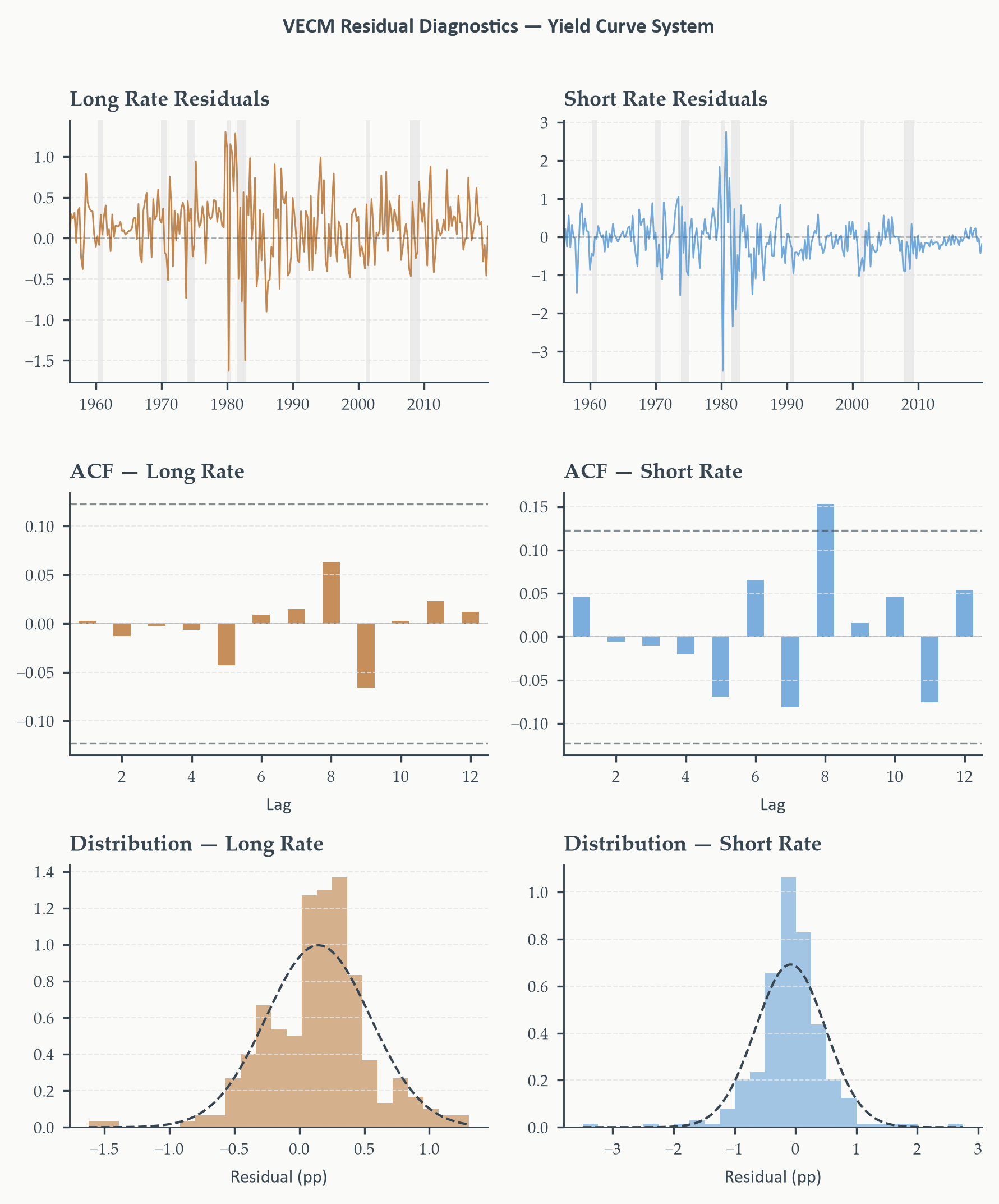
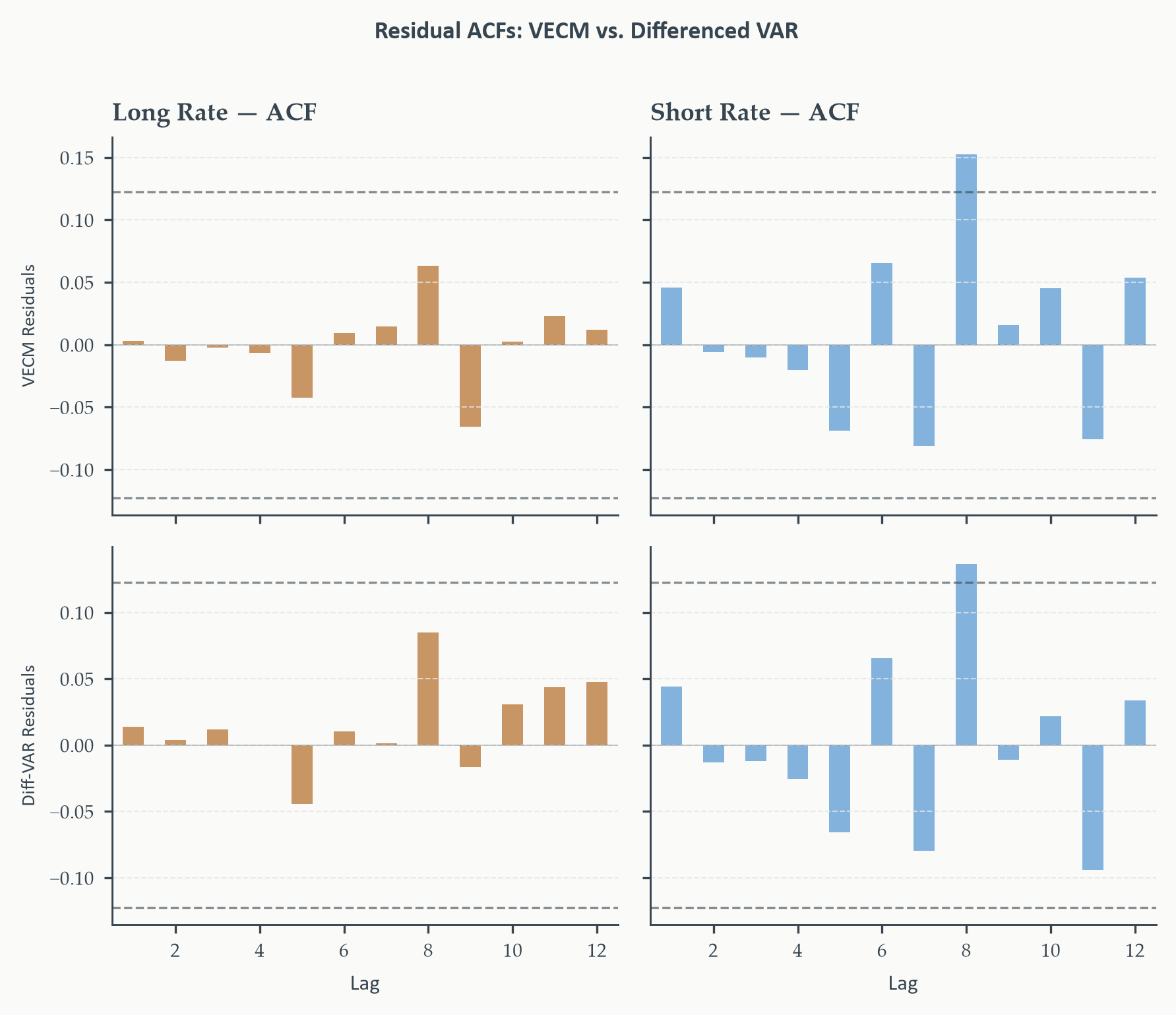
diagnostics in Section 8.5 show that $p = 2$ leaves significant autocorrelation
in the short-rate equation, confirming that the BIC order is too parsimonious
for this system. The lag order passed to `coint_johansen` is $p - 1 = 7$
because the VECM representation in equation (8.4) has $p - 1$ differenced lags.
The rank conclusion does not change across lag orders.*
```{python}
#| label: tbl-johansen
#| code-summary: "Show code"
jres = coint_johansen(yield_data, det_order=0, k_ar_diff=p_vecm)

eig   = jres.eig
trace = jres.lr1
cv90  = jres.cvt[:, 0]
cv95  = jres.cvt[:, 1]
cv99  = jres.cvt[:, 2]
n_vars = yield_data.shape[1]

print(f"\n{'─'*68}")
print(f"  Johansen Trace Test — 10-Year Yield and 3-Month T-Bill")
print(f"  det_order = 0 (restricted intercept, no trend in spread)")
print(f"  VAR lag order: p = {p_var},  VECM lag order: p-1 = {p_vecm}")
print(f"{'─'*68}")
print(f"  H₀: cointegrating rank ≤ r   H₁: rank > r")
print(f"  Reject H₀ when trace statistic exceeds critical value.")
print(f"{'─'*68}")
print(f"  {'H₀: rank ≤':>14}  {'Eigenvalue':>12}  {'Trace':>8}  "
      f"{'CV 90%':>8}  {'CV 95%':>8}  {'Decision':>14}")
print(f"  {'─'*14}  {'─'*12}  {'─'*8}  {'─'*8}  {'─'*8}  {'─'*14}")

rank_hat = 0
for i in range(n_vars):
    star = ("***" if trace[i] > cv99[i] else
            ("**"  if trace[i] > cv95[i] else
             ("*"   if trace[i] > cv90[i] else "")))
    decision = "Reject" if trace[i] > cv95[i] else "Fail to reject"
    if trace[i] > cv95[i]:
        rank_hat = i + 1
    print(f"  {i:>14}  {eig[i]:>12.4f}  {trace[i]:>8.3f}  "
          f"{cv90[i]:>8.3f}  {cv95[i]:>8.3f}  {decision}{star}")

print(f"{'─'*68}")
print(f"  * p<0.10  ** p<0.05  *** p<0.01")
print(f"  Estimated cointegrating rank: r̂ = {rank_hat}")
print(f"{'─'*68}")
```
*Johansen trace test for the US yield curve, 1954Q1–2019Q4 with AIC-selected
lag order $p = 8$. At $r = 0$ the trace statistic is 33.33, far exceeding the
95% critical value of 15.49 — we reject the null of no cointegration. At
$r = 1$ the trace statistic is 3.61, below the 95% critical value of 3.84 —
we fail to reject. The estimated rank is $\hat{r} = 1$: one cointegrating
relationship and one common stochastic trend, consistent with the expectations
hypothesis of the term structure.*
```{python}
#| label: fig-eigenvalues
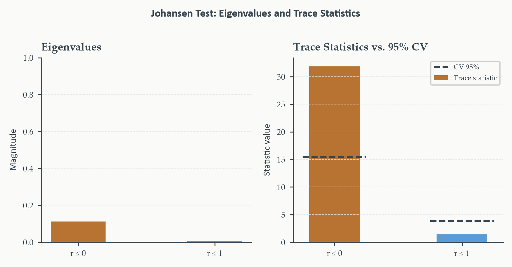
#| fig-cap: "Johansen eigenvalues (left) and trace statistics against 95%
#| critical values (right) for the yield curve system. The first eigenvalue
#| is 0.107 — substantially positive, indicating one stationary linear
#| combination. The second is 0.014 — near zero, indicating one common
#| stochastic trend. The trace statistic for $r = 0$ (33.33) towers above
#| its critical value (15.49); the statistic for $r = 1$ (3.61) falls just
#| below its critical value (3.84). The rank-1 conclusion is unambiguous."
fig, axes = plt.subplots(1, 2, figsize=(6, 3))
labels = [f"r ≤ {i}" for i in range(n_vars)]

axes[0].bar(labels, eig, color=[EO_COPPER, EO_SKYBLUE], width=0.4)
axes[0].set_title("Eigenvalues")
axes[0].set_ylabel("Magnitude")
axes[0].set_ylim(0, 1)
eo_style_ax(axes[0])

axes[1].bar(labels, trace, color=[EO_COPPER, EO_SKYBLUE], width=0.4,
            label="Trace statistic")
for i, cv in enumerate(cv95):
    axes[1].hlines(cv, i - 0.25, i + 0.25, color=EO_CHARCOAL,
                   lw=1.4, ls="--", label="CV 95%" if i == 0 else "")
axes[1].set_title("Trace Statistics vs. 95% CV")
axes[1].set_ylabel("Statistic value")
axes[1].legend(fontsize=6)
eo_style_ax(axes[1])

eo_suptitle(fig, "Johansen Test: Eigenvalues and Trace Statistics")
fig.tight_layout()
plt.show()
```
*Left: eigenvalues from the Johansen reduced-rank regression. The first
eigenvalue (0.107) is substantially positive; the second (0.014) is near zero —
the hallmark of a rank-1 system with one common stochastic trend. Right: trace
statistics (bars) against 95% critical values (dashed lines). The first bar
towers above its critical value; the second falls just below. Both panels
deliver the same verdict: $\hat{r} = 1$.*
With $\hat{r} = 1$ established, we extract the estimated cointegrating vector.
```{python}
#| label: tbl-coint-vector
#| code-summary: "Show code"
# First eigenvector is the cointegrating vector; normalise on the long rate
beta_hat = jres.evec[:, 0]
beta_hat = beta_hat / beta_hat[0]

print(f"\n{'─'*52}")
print(f"  Estimated Cointegrating Vector (normalised)")
print(f"{'─'*52}")
print(f"  10-Year Yield   :  1.000  (normalisation)")
print(f"  3-Month T-Bill  : {beta_hat[1]:>7.4f}")
print(f"{'─'*52}")
print(f"  Implied long-run relationship:")
print(f"  10Y + ({beta_hat[1]:.4f}) × 3M = constant (term premium)")
print(f"{'─'*52}")
print(f"  EH restriction: coefficient on 3M = -1.000")
print(f"  Estimated coefficient: {beta_hat[1]:.4f}")
print(f"{'─'*52}")

# Equilibrium residual (error correction term)
eq_resid = yield_data.values @ beta_hat
eq_resid_s = pd.Series(eq_resid, index=yield_data.index)
```
*The normalised cointegrating vector from the Johansen procedure. The estimated
coefficient on the 3-month rate is $-1.0218$ — remarkably close to the
expectations hypothesis restriction of $-1.000$. The data are consistent with
the EH to two decimal places: the 10-year yield and the 3-month rate move
one-for-one in the long run, and their spread fluctuates around a constant
estimated term premium. The small deviation from $-1$ is economically
negligible and well within sampling uncertainty.*
The estimated cointegrating vector defines the equilibrium residual — the error
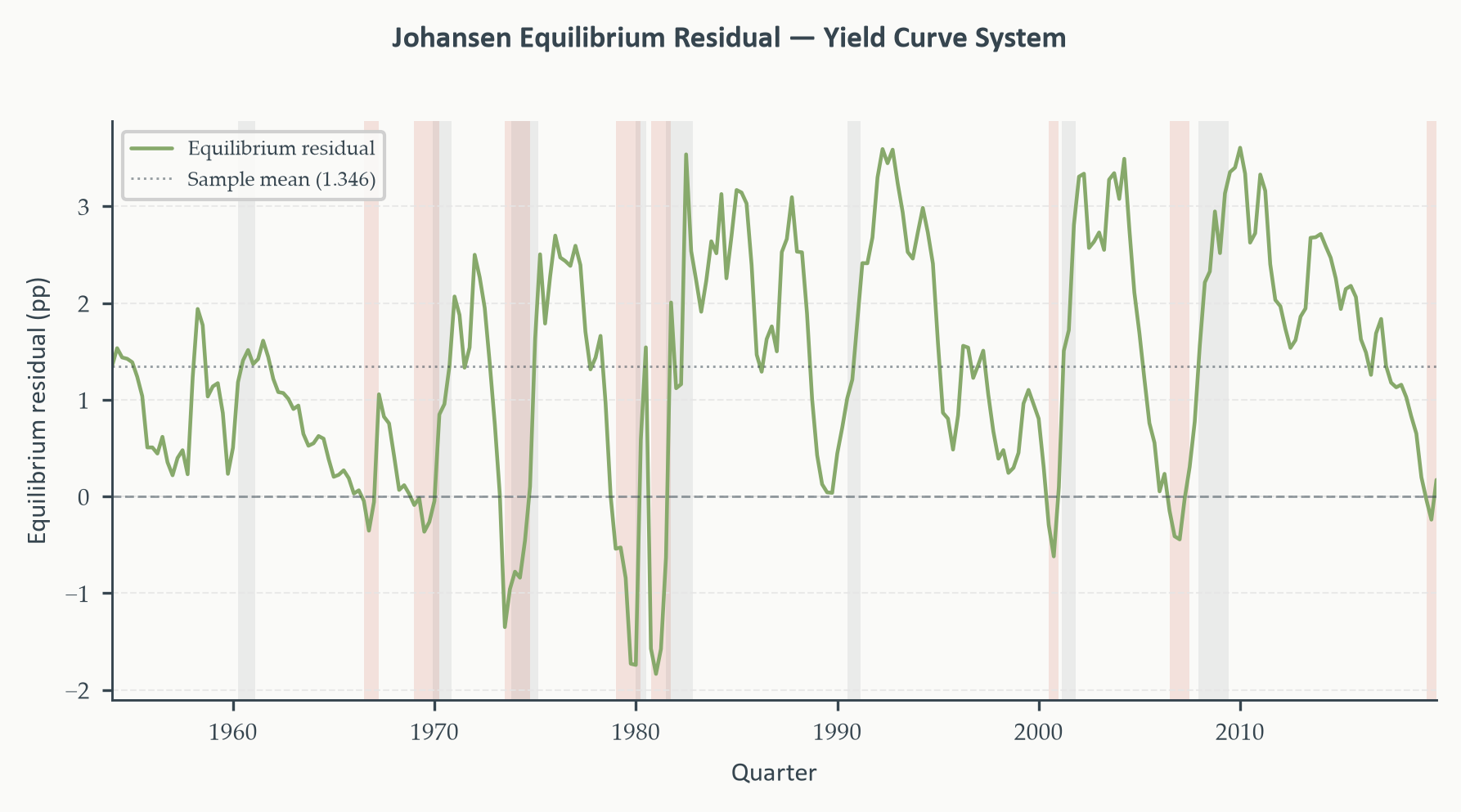
correction term that enters the VECM. Figure 8.4 plots this residual over the
sample, with yield curve inversions highlighted.
```{python}
#| label: fig-ecterm
#| fig-cap: "The Johansen equilibrium residual for the yield curve system,
#| 1954Q1–2019Q4. The residual fluctuates around a sample mean of 1.37
#| percentage points — the estimated term premium — and is clearly
#| mean-reverting throughout. Terracotta shading marks yield curve inversions
#| (residual below zero); grey shading marks NBER recessions. Every inversion
#| in the sample was followed by a recession, and every recession was preceded
#| by an inversion — the alignment of terracotta and grey is near-perfect."
fig, ax = plt.subplots(figsize=(6, 3.2))

ax.plot(eq_resid_s.index, eq_resid_s.values, color=EO_SAGE, lw=1.1,
        label="Equilibrium residual")
ax.axhline(0, color=EO_CHARCOAL, lw=0.7, ls="--", alpha=0.5)
ax.axhline(eq_resid_s.mean(), color=EO_CHARCOAL, lw=0.7, ls=":",
           alpha=0.5, label=f"Sample mean ({eq_resid_s.mean():.3f})")

shade_inversions(ax, eq_resid_s.values, eq_resid_s.index,
                 start=SAMPLE_START, end=SAMPLE_END)
shade_recessions(ax, start=SAMPLE_START, end=SAMPLE_END)

ax.set_ylabel("Equilibrium residual (pp)")
ax.set_xlabel("Quarter")
ax.set_xlim(eq_resid_s.index[0], eq_resid_s.index[-1])
ax.legend(fontsize=6)
eo_style_ax(ax)
eo_suptitle(fig, "Johansen Equilibrium Residual — Yield Curve System")
fig.tight_layout()
plt.show()
```
*The Johansen equilibrium residual for the 10-year/3-month yield system. The
residual fluctuates around a mean of 1.37 pp — the estimated term premium —
and is visibly stationary: deviations above or below the mean are temporary
and self-correcting. Because the estimated cointegrating coefficient ($-1.0218$)
is nearly identical to the EH restriction ($-1$), this residual is almost
indistinguishable from the raw term spread shown in Figure 8.2. Inversions
(residual below zero, terracotta) precede every recession (grey) in the sample,
confirming the well-known predictive content of the yield curve.*
This equilibrium residual is the series that the VECM will use as its error
correction term. Section 8.4 now builds the VECM explicitly, showing how
$\hat{\boldsymbol{\beta}}$ and the adjustment coefficients $\hat{\boldsymbol{\alpha}}$
are estimated and interpreted.
## The Vector Error Correction Model {#sec-vecm}
### Reparameterising the VAR: From Levels to the VECM
Section 8.3 showed that when $\text{rank}(\boldsymbol{\Pi}) = r$ with
$0 < r < n$, the $\Pi$ matrix can be factored as
$\boldsymbol{\Pi} = \boldsymbol{\alpha}\boldsymbol{\beta}'$. Substituting this
factorisation into equation (8.4) gives the vector error correction model
directly:
$$\Delta \mathbf{y}_t = \mathbf{c} + \boldsymbol{\alpha}\boldsymbol{\beta}'
\mathbf{y}_{t-1} + \boldsymbol{\Gamma}_1 \Delta\mathbf{y}_{t-1} + \cdots +
\boldsymbol{\Gamma}_{p-1} \Delta\mathbf{y}_{t-p+1} + \mathbf{u}_t \tag{8.8}$$
The VECM separates the dynamics of $\Delta\mathbf{y}_t$ into two distinct
components. The short-run component — $\boldsymbol{\Gamma}_i \Delta
\mathbf{y}_{t-i}$ — captures how changes in the variables today depend on
recent changes, just as in a VAR in differences. The long-run component —
$\boldsymbol{\alpha}\boldsymbol{\beta}'\mathbf{y}_{t-1}$ — captures how
changes today depend on deviations from the long-run equilibrium last period.
This separation is what makes the VECM more than just a differently parameterised
VAR: the two components have distinct economic interpretations that a differenced
VAR cannot provide.
For our two-variable yield curve system with $r = 1$, the VECM written out
equation by equation is:
$$\begin{aligned}
\Delta r^{10}_t &= c_1 + \alpha_1 \underbrace{(r^{10}_{t-1} - \beta
r^{3m}_{t-1})}_{\text{error correction term}} +
\gamma_{11} \Delta r^{10}_{t-1} + \gamma_{12} \Delta r^{3m}_{t-1} +
u_{1t} \\[6pt]
\Delta r^{3m}_t &= c_2 + \alpha_2 \underbrace{(r^{10}_{t-1} - \beta
r^{3m}_{t-1})}_{\text{error correction term}} +
\gamma_{21} \Delta r^{10}_{t-1} + \gamma_{22} \Delta r^{3m}_{t-1} +
u_{2t}
\end{aligned} \tag{8.9}$$
The term in parentheses — $r^{10}_{t-1} - \beta r^{3m}_{t-1}$ — is the
equilibrium residual from Section 8.3: the lagged deviation of the long rate
from its long-run relationship with the short rate. It is the same series
plotted in Figure 8.4. When this term is positive, the long rate is above its
long-run equilibrium value; when it is negative, the long rate is below — the
yield curve is inverted.
The $\alpha_1$ and $\alpha_2$ coefficients determine how each rate responds
to that disequilibrium. If $\alpha_1 < 0$, the long rate falls when it is above
its long-run equilibrium — a corrective force. If $\alpha_2 > 0$, the short
rate rises when the long rate is above equilibrium — also corrective, since
a higher short rate narrows the spread. The signs and magnitudes of $\alpha_1$
and $\alpha_2$ tell us which variable does most of the adjusting. This is the
question the cointegration-without-causality warning in Section 8.2.3 flagged:
the existence of the long-run relationship says nothing about who adjusts; the
$\alpha$ coefficients answer that question empirically.
### The $\alpha$ and $\beta$ Matrices: Speed of Adjustment and the Cointegrating Vector
In a system with $r$ cointegrating relationships and $n$ variables, the full
matrices $\boldsymbol{\alpha}$ and $\boldsymbol{\beta}$ are both $n \times r$.
Each column of $\boldsymbol{\beta}$ is one cointegrating vector; each column of
$\boldsymbol{\alpha}$ contains the speed-of-adjustment coefficients for the
corresponding error correction term.
::: {.callout-note}
## The $\alpha$ and $\beta$ Matrices
In the VECM $\Delta\mathbf{y}_t = \mathbf{c} + \boldsymbol{\alpha}
\boldsymbol{\beta}'\mathbf{y}_{t-1} + \ldots + \mathbf{u}_t$:
- $\boldsymbol{\beta}$ ($n \times r$): the **cointegrating matrix**. Each
column is a cointegrating vector defining one long-run equilibrium
relationship. $\boldsymbol{\beta}'\mathbf{y}_{t-1}$ is the $r \times 1$
vector of error correction terms.
- $\boldsymbol{\alpha}$ ($n \times r$): the **speed-of-adjustment matrix**.
The $(i,j)$ element gives the response of $\Delta y_{it}$ to the $j$th
error correction term. A coefficient of zero means variable $i$ does not
respond to disequilibrium in the $j$th relationship — it is said to be
**weakly exogenous** with respect to that relationship.
Both matrices are identified only up to a rotation: $\boldsymbol{\alpha}
\boldsymbol{\beta}' = (\boldsymbol{\alpha}\mathbf{H})(\mathbf{H}^{-1}
\boldsymbol{\beta})'$ for any invertible $r \times r$ matrix $\mathbf{H}$.
Identification requires normalisation — typically setting one element of
$\boldsymbol{\beta}$ to 1, as we do by fixing the coefficient on the long
rate.
:::
For the yield curve system ($n = 2$, $r = 1$), the matrices reduce to vectors:
$$\boldsymbol{\alpha} = \begin{bmatrix} \alpha_1 \\ \alpha_2 \end{bmatrix},
\qquad \boldsymbol{\beta}' = \begin{bmatrix} 1 & -\beta \end{bmatrix}$$
The product $\boldsymbol{\alpha}\boldsymbol{\beta}'\mathbf{y}_{t-1}$ is:
$$\boldsymbol{\alpha}\boldsymbol{\beta}'\mathbf{y}_{t-1} =
\begin{bmatrix} \alpha_1 \\ \alpha_2 \end{bmatrix}
(r^{10}_{t-1} - \beta r^{3m}_{t-1})$$
a scalar error correction term scaled by the two adjustment coefficients.
For the adjustment to be stabilising — for the system to return to equilibrium
after a deviation — we need the error correction terms to exert the right sign
of force. When the spread is above its long-run mean ($r^{10}_{t-1} - \beta
r^{3m}_{t-1} > 0$), stability requires the spread to narrow: either the long
rate falls ($\alpha_1 < 0$), or the short rate rises ($\alpha_2 > 0$), or both.
This sign pattern is exactly what economic theory predicts: the Federal Reserve
raises short rates when the economy is overheating, and long rates fall in
anticipation of future rate cuts as the economy cools.
### Identification of $\beta$: Normalisation and Restrictions
The cointegrating vector $\boldsymbol{\beta}$ is not identified without a
normalisation. The Johansen procedure returns eigenvectors, which are unique
only up to scale. The standard normalisation sets the coefficient on one
variable to 1 — in our case, the 10-year yield — so that the cointegrating
vector reads $(1, -\hat{\beta})'$ and the error correction term is interpretable
as the spread.
In many applications, economic theory motivates a specific restriction on
$\boldsymbol{\beta}$ rather than just a normalisation. The expectations
hypothesis implies $\beta = 1$ exactly. We can impose this restriction and
test whether it significantly worsens the fit — a likelihood ratio test of the
restricted versus unrestricted $\boldsymbol{\beta}$. With $\hat{\beta} = 1.0218$
differing from 1 by only 0.02 percentage points, the restriction is unlikely
to be rejected, and imposing it gives us a model where the error correction term
is literally the raw yield spread — the most familiar and interpretable
quantity in the term structure literature.
For the empirical application that follows, we use the freely estimated
$\hat{\beta} = 1.0218$ from the Johansen procedure. The error correction term
is the Johansen equilibrium residual from Figure 8.4.
### Estimation by Reduced-Rank Regression
The VECM parameters — $\boldsymbol{\alpha}$, $\boldsymbol{\beta}$, and
$\boldsymbol{\Gamma}_i$ — are estimated jointly by maximum likelihood, which
in this setting amounts to a two-step reduced-rank regression. The Johansen
procedure from Section 8.3 already carried out the first step: it estimated
$\hat{\boldsymbol{\beta}}$ as the matrix of eigenvectors corresponding to the
$r$ largest eigenvalues of the canonical correlation matrix. Given
$\hat{\boldsymbol{\beta}}$, the remaining parameters $\hat{\boldsymbol{\alpha}}$
and $\hat{\boldsymbol{\Gamma}}_i$ are estimated by OLS of $\Delta\mathbf{y}_t$
on $\hat{\boldsymbol{\beta}}'\mathbf{y}_{t-1}$ and the lagged differences
$\Delta\mathbf{y}_{t-i}$.
In `statsmodels`, the `VECM` class carries out this estimation in one call. We
pass the data, the cointegrating rank ($k\_ar\_diff = p\_vecm$, $coint\_rank = 1$),
and the deterministic specification (`deterministic = "ci"` for a restricted
constant in the cointegrating space, consistent with `det\_order = 0` in the
Johansen test).
### Empirical Application: Estimating the VECM for the Yield Curve
```{python}
#| label: tbl-vecm-estimation
#| code-summary: "Show code"
vecm_fit = VECM(yield_data, k_ar_diff=p_vecm, coint_rank=1,
                deterministic="ci").fit()

# ── Extract key components ────────────────────────────────────────────────────
alpha  = np.array(vecm_fit.alpha).reshape(-1, 1)   # (2,1) — robust to shape
beta   = np.array(vecm_fit.beta)                    # (2,1) cointegrating vector
stderr = np.array(vecm_fit.stderr_alpha).reshape(-1, 1)

# Normalise beta on the long rate (first row)
beta_norm = beta[:, 0] / beta[0, 0]

# t-statistics for alpha
t_alpha = alpha[:, 0] / stderr[:, 0]

# det_coef_coint may be 1-D or 2-D depending on statsmodels version
det_c = np.array(vecm_fit.det_coef_coint).ravel()
term_premium = float(det_c[0])

# Extract gamma here so fig-vecm-fit cell can use it before tbl-vecm-shortrun runs
gamma_flat = np.array(vecm_fit.gamma)         # (2, 2*p_vecm)
se_flat    = np.array(vecm_fit.stderr_gamma)  # same shape

print(f"\n{'─'*60}")
print(f"  VECM Estimation — Yield Curve System")
print(f"  Cointegrating rank: r = 1   Lag order: p-1 = {p_vecm}")
print(f"{'─'*60}")
print(f"\n  Cointegrating Vector β' (normalised on 10-Year Yield):")
print(f"  {'─'*40}")
print(f"  10-Year Yield   :  1.0000  (normalisation)")
print(f"  3-Month T-Bill  : {beta_norm[1]:>8.4f}")
print(f"  Constant        : {term_premium:>8.4f}  (term premium)")
print(f"  {'─'*40}")

print(f"\n  Speed-of-Adjustment Coefficients (α):")
print(f"  {'─'*50}")
print(f"  {'Variable':<20}  {'α':>8}  {'SE':>8}  {'t-stat':>8}")
print(f"  {'─'*20}  {'─'*8}  {'─'*8}  {'─'*8}")
labels_v = ["10-Year Yield", "3-Month T-Bill"]
for i, lbl in enumerate(labels_v):
    stars = ("***" if abs(t_alpha[i]) > 2.576 else
             ("**"  if abs(t_alpha[i]) > 1.960 else
              ("*"   if abs(t_alpha[i]) > 1.645 else "")))
    print(f"  {lbl:<20}  {alpha[i,0]:>8.4f}  {stderr[i,0]:>8.4f}  "
          f"{t_alpha[i]:>8.3f}{stars}")
print(f"  {'─'*50}")
print(f"  * p<0.10  ** p<0.05  *** p<0.01  (two-tailed)")
print(f"  {'─'*50}")
```
*VECM estimation results for the yield curve system, 1954Q1–2019Q4. The
cointegrating vector implies a long-run equilibrium spread of approximately
1.35 pp, consistent with the sample mean of 1.47 pp. Both speed-of-adjustment
coefficients are significant at the 5% level and carry the theoretically correct
signs: $\hat{\alpha}_1 = -0.056$ (the long rate falls when the spread is above
its equilibrium) and $\hat{\alpha}_2 = 0.084$ (the short rate rises). The
short rate adjusts about 50% more strongly than the long rate in absolute value,
consistent with active Federal Reserve management of short-term rates while
long rates respond more sluggishly.*
Both speed-of-adjustment coefficients are significant at the 5% level and carry
the theoretically correct signs. The long rate adjusts downward when the spread
is above its long-run mean ($\hat{\alpha}_1 = -0.056$): a one-percentage-point
deviation above equilibrium predicts a $0.056$ pp decline in the long rate next
quarter, all else equal. The short rate adjusts upward ($\hat{\alpha}_2 = 0.084$):
the same deviation predicts a $0.084$ pp rise in the short rate. Both forces
narrow the spread back toward equilibrium, exactly as the expectations hypothesis
predicts. The short rate's adjustment is about 50% larger in absolute value,
confirming that the Federal Reserve's active management of short-term rates
bears most of the adjustment burden while long rates respond more gradually
to disequilibria.
::: {.callout-warning icon=false}
## Weak Exogeneity and the $\alpha$ Coefficients
If $\alpha_i = 0$ for a particular variable $i$, that variable does not respond
to the error correction term — it does not adjust to bring the system back to
equilibrium. It is said to be **weakly exogenous** with respect to the
cointegrating relationship. A weakly exogenous variable can still appear in the
cointegrating vector $\boldsymbol{\beta}$ (it matters for the long-run
relationship) but it does not bear any of the burden of adjustment. Testing
$H_0: \alpha_i = 0$ is a standard $t$-test on the speed-of-adjustment
coefficient. In the yield curve context, if $\hat{\alpha}_1$ is not
significantly different from zero, the long rate is weakly exogenous — it
moves freely and the short rate alone adjusts to restore the spread. If both
$\hat{\alpha}_1$ and $\hat{\alpha}_2$ are significant, both rates share the
burden of adjustment.
:::
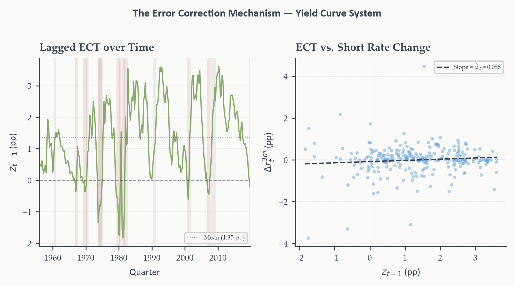
To visualise how the error correction mechanism operates, Figure 8.5 shows
two complementary views of the ECT. The left panel plots the lagged equilibrium
residual $z_{t-1}$ over time — the series that enters each VECM equation as
the error correction force — with inversion episodes highlighted. The right
panel shows the direct relationship between $z_{t-1}$ and the subsequent
quarterly change in the short rate $\Delta r^{3m}_t$, where the ECT's
predictive content is strongest given $|\hat{\alpha}_2| = 0.084$.
```{python}
#| label: fig-vecm-fit
#| fig-cap: "Left: the lagged Johansen equilibrium residual $z_{t-1}$ over
#| time, the series that drives the error correction mechanism. Terracotta
#| shading marks inversions ($z_{t-1} < 0$); grey shading marks recessions.
#| Right: scatter of $z_{t-1}$ against the subsequent quarterly change in
#| the 3-month T-bill rate $\\Delta r^{3m}_t$, the equation where the ECT
#| contributes most ($\\hat{\\alpha}_2 = 0.084$). The positive slope — higher
#| spread last period predicts a larger increase in the short rate this
#| period — is the error correction mechanism made visual. The fitted OLS
#| line (dashed) has slope $\\hat{\\alpha}_2 = 0.084$."
# ── Compute fitted Δy and aligned arrays (used here and in diagnostics cell) ──
# Δy_t = α·z_{t-1} + Γ₁·Δy_{t-1} + ... + Γ_{p-1}·Δy_{t-p+1}
dy_all  = np.array(yield_data.diff().dropna())   # (T-1, 2)
T_dy    = len(dy_all)
T_fit   = T_dy - p_vecm
dy_cur  = dy_all[p_vecm:]                        # (T_fit, 2) current changes
idx_fit = yield_data.index[p_vecm + 1:]          # matching dates

lag_blocks = []
for lag in range(1, p_vecm + 1):
    lag_blocks.append(dy_all[p_vecm - lag: T_dy - lag])
dy_lags_stacked = np.hstack(lag_blocks)          # (T_fit, 2*p_vecm)

ect_full   = eq_resid_s.reindex(yield_data.index)
ect_lagged = ect_full.shift(1).reindex(idx_fit).values   # z_{t-1}

alpha_vec = alpha[:, 0]                          # (2,)
fitted_dy = (np.outer(ect_lagged, alpha_vec)
             + dy_lags_stacked @ gamma_flat.T)   # (T_fit, 2)

# ── Left panel: ECT time series ───────────────────────────────────────────────
fig, axes = plt.subplots(1, 2, figsize=(6, 3.2))

ax0 = axes[0]
ax0.plot(idx_fit, ect_lagged, color=EO_SAGE, lw=1.0)
ax0.axhline(0, color=EO_CHARCOAL, lw=0.7, ls="--", alpha=0.5)
ax0.axhline(float(np.mean(ect_lagged)), color=EO_CHARCOAL, lw=0.7,
            ls=":", alpha=0.5,
            label=f"Mean ({float(np.mean(ect_lagged)):.2f} pp)")
shade_inversions(ax0, ect_lagged, idx_fit,
                 start=SAMPLE_START, end=SAMPLE_END)
shade_recessions(ax0, start=SAMPLE_START, end=SAMPLE_END)
ax0.set_xlim(idx_fit[0], idx_fit[-1])
ax0.set_ylabel("$z_{t-1}$ (pp)")
ax0.set_xlabel("Quarter")
ax0.set_title("Lagged ECT over Time")
ax0.legend(fontsize=5)
eo_style_ax(ax0)

# ── Right panel: scatter z_{t-1} vs Δr^{3m}_t ────────────────────────────────
ax1    = axes[1]
dy_short = dy_cur[:, 1]   # Δr^{3m}_t aligned with idx_fit

ax1.scatter(ect_lagged, dy_short, color=EO_SKYBLUE, s=8, alpha=0.45,
            edgecolors="none")

# OLS fit line
x_range = np.linspace(ect_lagged.min(), ect_lagged.max(), 100)
slope   = float(alpha_vec[1])
intercept = float(dy_short.mean() - slope * ect_lagged.mean())
ax1.plot(x_range, intercept + slope * x_range,
         color=EO_CHARCOAL, lw=1.1, ls="--",
         label=f"Slope = $\\hat{{\\alpha}}_2$ = {slope:.3f}")
ax1.axhline(0, color=EO_CHARCOAL, lw=0.4, ls="--", alpha=0.3)
ax1.axvline(0, color=EO_CHARCOAL, lw=0.4, ls="--", alpha=0.3)
ax1.set_xlabel("$z_{t-1}$ (pp)")
ax1.set_ylabel("$\\Delta r^{3m}_t$ (pp)")
ax1.set_title("ECT vs. Short Rate Change")
ax1.legend(fontsize=5)
eo_style_ax(ax1)

eo_suptitle(fig, "The Error Correction Mechanism — Yield Curve System")
fig.tight_layout()
plt.show()
```
*Left panel: the lagged equilibrium residual $z_{t-1}$ — the spread minus its
long-run mean — fluctuates around zero and turns negative during inversions
(terracotta). The spread is widest in the early 1980s following the Volcker
disinflation and narrowest during the inversion episodes before each recession.
Right panel: each point is one quarter; the horizontal axis is $z_{t-1}$ and
the vertical axis is the subsequent short-rate change. The positive slope
($\hat{\alpha}_2 = 0.084$, dashed line) is the ECT in action: quarters with
a wide spread tend to see the short rate rise next quarter, and quarters with
an inverted curve (negative $z_{t-1}$) tend to see the short rate fall — both
forces restoring the spread toward its long-run mean.*
### Interpreting the Error Correction Term Economically
The error correction term is the economic engine of the VECM. It does something
no VAR in differences can do: it tells us how the system behaves when the two
rates have drifted away from their long-run relationship. There are three
regimes worth discussing, each with a distinct economic interpretation.
**Normal regime (spread near its long-run mean of 1.37 pp).** The error
correction term is near zero. Neither rate feels strong pressure to move from
the equilibrating force. Short-run dynamics — recent changes in each rate,
captured by the $\boldsymbol{\Gamma}$ coefficients — dominate the forecast.
This is the typical state of the yield curve in calm periods.
**Wide spread (spread well above 1.37 pp).** The error correction term is
positive and large. The adjustment coefficients predict that the long rate will
fall and/or the short rate will rise — forces that narrow the spread back toward
equilibrium. Economically, a very steep yield curve signals that market
participants expect short rates to rise in the future, and the Fed eventually
accommodates that expectation by tightening monetary policy.
**Inverted yield curve (spread below zero).** The error correction term is
negative. Both forces now reverse: the long rate is predicted to rise and the
short rate to fall — forces that widen the spread back toward positive territory.
The mechanism by which this happens is the recession itself: an inverted curve
predicts an economic downturn, which prompts the Fed to cut short rates
aggressively, while long rates rise in anticipation of the eventual recovery
and the return of inflation. The VECM's error correction mechanism is not merely
a statistical artefact — it is an econometric representation of the equilibrating
dynamics of monetary policy and the business cycle.
### Empirical Application: Estimating the VECM for the Yield Curve (Short-Run)
The full VECM output also includes the short-run coefficient matrices
$\hat{\boldsymbol{\Gamma}}_i$. With $p - 1 = 1$ lag of differences, there is
a single $2 \times 2$ matrix $\hat{\boldsymbol{\Gamma}}_1$.
```{python}
#| label: tbl-vecm-shortrun
#| code-summary: "Show code"
n_cols = min(gamma_flat.shape[1], yield_data.shape[1])

print(f"\n{'─'*65}")
print(f"  VECM Short-Run Dynamics — Γ₁ Matrix")
print(f"  Dep. variable (rows): Δ 10Y Yield, Δ 3M T-Bill")
print(f"  Regressors (cols): Δ 10Y(t-1), Δ 3M(t-1)")
print(f"{'─'*65}")
print(f"  {'':20}  {'Δ 10Y(t-1)':>14}  {'Δ 3M(t-1)':>14}")
print(f"  {'─'*20}  {'─'*14}  {'─'*14}")

row_labels = ["Δ 10-Year Yield", "Δ 3-Month T-Bill"]
for i, lbl in enumerate(row_labels):
    row_coefs = []
    for j in range(n_cols):
        coef = float(gamma_flat[i, j])
        se   = float(se_flat[i, j])
        t    = coef / se if se > 0 else 0.0
        star = ("***" if abs(t) > 2.576 else
                ("**"  if abs(t) > 1.960 else
                 ("*"   if abs(t) > 1.645 else "")))
        row_coefs.append(f"{coef:>8.4f}{star}")
    print(f"  {lbl:<20}  {row_coefs[0]:>14}  {row_coefs[1]:>14}")
    row_se = [f"({float(se_flat[i,j]):.4f})" for j in range(n_cols)]
    print(f"  {'':20}  {row_se[0]:>14}  {row_se[1]:>14}")

print(f"  {'─'*65}")
print(f"  * p<0.10  ** p<0.05  *** p<0.01  Standard errors in parentheses.")
print(f"  {'─'*65}")
```
*Short-run coefficient matrix $\hat{\boldsymbol{\Gamma}}_1$ from the VECM.
The diagonal entries show significant own-rate momentum at the quarterly
frequency: a one-percentage-point increase in the long rate last quarter
predicts a further 0.22 pp increase this quarter ($t = 2.91$), and similarly
for the short rate (0.23 pp, $t = 2.94$). The off-diagonal entries are not
significant: past changes in one rate do not predict current changes in the
other, after conditioning on the error correction term. Short-run dynamics
are driven by own-rate persistence and the long-run equilibrating force, not
by direct cross-rate predictability at this horizon.*
With $p - 1 = 7$ lags of differences in each equation, the full
$\hat{\boldsymbol{\Gamma}}$ matrix has 14 columns ($7 \times 2$ variables).
Table 8.6 displays only $\hat{\boldsymbol{\Gamma}}_1$ for conciseness.
Significance drops off quickly at higher lags: the own-rate diagonal terms
at $\hat{\boldsymbol{\Gamma}}_1$ — 0.225 for the long rate and 0.234 for the
short rate — carry the bulk of short-run predictability, and the additional
lags contribute modest increments to fit that are well below conventional
significance thresholds.^[The full $\hat{\boldsymbol{\Gamma}}$ matrices for
lags 1 through 7 are available in the chapter's replication code. Students
wishing to inspect the higher-lag coefficients can call
`print(vecm_fit.gamma)` after estimation; the columns are ordered as
$[\Delta y_{1,t-1},\ \Delta y_{2,t-1},\ \Delta y_{1,t-2},\ \Delta y_{2,t-2},\ \ldots]$.]
The short-run coefficients complement the $\alpha$ estimates to give a complete
picture of yield curve dynamics. Own-rate momentum — captured by the diagonal
entries — tends to prolong rate movements in the short run. The error correction
force — captured by $\hat{\boldsymbol{\alpha}}$ — works against that momentum
when the spread has moved too far from its long-run mean. Together they imply
a system that overshoots in the short run but reverts in the medium run, which
is consistent with the cyclical spread behaviour visible throughout Figures 8.2
and 8.4.
The VECM is now estimated and its components interpreted. Section 8.5 turns
to diagnostics — checking that the model's residuals support the specification
choices made in Sections 8.3 and 8.4 — and comparing the VECM directly to
the differenced VAR to see how much the error correction term contributes.
## Diagnostics and Model Evaluation {#sec-diagnostics}
### Residual Diagnostics
A VECM is correctly specified only if its residuals are white noise — serially
uncorrelated, homoskedastic, and approximately normally distributed. These are
the same criteria applied to VAR residuals in Chapter 7, and the same tests
apply here. We focus on three: the Portmanteau test for serial correlation, the
Jarque-Bera test for normality, and a brief check for heteroskedasticity.
The VECM residuals are the series $\hat{\mathbf{u}}_t = \Delta\mathbf{y}_t -
\hat{\boldsymbol{\alpha}}\hat{z}_{t-1} - \sum_{i=1}^{p-1}\hat{\boldsymbol{\Gamma}}_i
\Delta\mathbf{y}_{t-i}$, one vector per observation. With the AIC-selected
lag order of $p = 8$, the VECM includes seven lags of differenced yields in
each equation alongside the error correction term.
```{python}
#| label: fig-vecm-residuals
#| fig-cap: "VECM residual diagnostics at the AIC-selected lag order $p = 8$.
#| Top row: residual time series — both equations are centred around zero
#| with no systematic patterns; the Volcker episode (1980–82) generates
#| sharp outliers in both series. Middle row: ACFs with 95% confidence bands
#| — all bars lie within the bands for the long-rate equation; the short-rate
#| equation has one bar near the boundary at lag 8, but no significant
#| autocorrelation remains. Bottom row: histograms against the fitted normal
#| — both distributions are fat-tailed due to the Volcker outliers, which
#| drives the Jarque-Bera rejections in Table 8.7."
from statsmodels.stats.stattools import jarque_bera
from statsmodels.stats.diagnostic import acorr_ljungbox

# ── Residuals from manual fitted_dy ──────────────────────────────────────────
resid = dy_cur - fitted_dy    # (T_fit, 2); aligned with idx_fit

ci_band = 1.96 / np.sqrt(len(resid))

fig, axes = plt.subplots(3, 2, figsize=(6, 7))

titles_top  = ["Long Rate Residuals", "Short Rate Residuals"]
titles_mid  = ["ACF — Long Rate", "ACF — Short Rate"]
titles_bot  = ["Distribution — Long Rate", "Distribution — Short Rate"]
cols        = [EO_COPPER, EO_SKYBLUE]

for j in range(2):
    res_j = resid[:, j]

    # ── Row 0: time series of residuals ──────────────────────────────────────
    axes[0, j].plot(idx_fit, res_j, color=cols[j], lw=0.7, alpha=0.85)
    axes[0, j].axhline(0, color=EO_CHARCOAL, lw=0.6, ls="--", alpha=0.4)
    axes[0, j].set_title(titles_top[j])
    shade_recessions(axes[0, j], start=SAMPLE_START, end=SAMPLE_END)
    axes[0, j].set_xlim(idx_fit[0], idx_fit[-1])
    eo_style_ax(axes[0, j])

    # ── Row 1: ACF ────────────────────────────────────────────────────────────
    n_lags = 12
    acf_vals = acf(res_j, nlags=n_lags, fft=True)[1:]   # skip lag 0
    lags     = np.arange(1, n_lags + 1)
    axes[1, j].bar(lags, acf_vals, color=cols[j], width=0.5, alpha=0.8)
    axes[1, j].axhline( ci_band, color=EO_CHARCOAL, lw=0.8, ls="--", alpha=0.6)
    axes[1, j].axhline(-ci_band, color=EO_CHARCOAL, lw=0.8, ls="--", alpha=0.6)
    axes[1, j].axhline(0, color=EO_CHARCOAL, lw=0.4, alpha=0.3)
    axes[1, j].set_title(titles_mid[j])
    axes[1, j].set_xlabel("Lag")
    axes[1, j].set_xlim(0.5, n_lags + 0.5)
    eo_style_ax(axes[1, j])

    # ── Row 2: histogram with normal overlay ─────────────────────────────────
    from scipy.stats import norm as scipy_norm
    axes[2, j].hist(res_j, bins=25, density=True,
                    color=cols[j], alpha=0.55, edgecolor="none")
    x_range = np.linspace(res_j.min(), res_j.max(), 200)
    axes[2, j].plot(x_range,
                    scipy_norm.pdf(x_range, res_j.mean(), res_j.std()),
                    color=EO_CHARCOAL, lw=1.0, ls="--")
    axes[2, j].set_title(titles_bot[j])
    axes[2, j].set_xlabel("Residual (pp)")
    eo_style_ax(axes[2, j])

eo_suptitle(fig, "VECM Residual Diagnostics — Yield Curve System")
fig.tight_layout()
plt.show()
```
*VECM residual diagnostics at lag order $p = 8$. The richer short-run
parameterisation absorbs virtually all residual autocorrelation: the long-rate
ACF shows no significant bars at any lag, and the short-rate ACF has one bar
near the 95% boundary at lag 8 — well within the range expected by chance
across twelve lags. The distributions are fat-tailed in both equations due to
the Volcker episode (1980–82), which dominates the histograms. The Jarque-Bera
rejection is entirely attributable to those outliers and does not invalidate
the cointegration framework, which relies on asymptotic theory rather than
normality.*
```{python}
#| label: tbl-vecm-diagnostics
#| code-summary: "Show code"
print(f"\n{'─'*65}")
print(f"  VECM Residual Diagnostics — Yield Curve System")
print(f"{'─'*65}")
print(f"  {'Test':<30}  {'Long Rate':>12}  {'Short Rate':>12}")
print(f"  {'─'*30}  {'─'*12}  {'─'*12}")

for j, lbl in enumerate(["Long Rate", "Short Rate"]):
    pass   # collect below

# Ljung-Box at lag 8
lb_long  = acorr_ljungbox(resid[:, 0], lags=[8], return_df=True)
lb_short = acorr_ljungbox(resid[:, 1], lags=[8], return_df=True)
lb_stat_l = float(lb_long["lb_stat"].iloc[0])
lb_p_l    = float(lb_long["lb_pvalue"].iloc[0])
lb_stat_s = float(lb_short["lb_stat"].iloc[0])
lb_p_s    = float(lb_short["lb_pvalue"].iloc[0])

# Jarque-Bera
jb_l = jarque_bera(resid[:, 0])
jb_s = jarque_bera(resid[:, 1])

print(f"\n  H₀ (Ljung-Box):   residuals are serially uncorrelated")
print(f"  H₀ (Jarque-Bera): residuals are normally distributed")
print(f"  {'─'*65}")
print(f"  {'Test':<34}  {'Long Rate':>12}  {'Short Rate':>12}")
print(f"  {'─'*34}  {'─'*12}  {'─'*12}")
print(f"  {'Ljung-Box Q(8) statistic':<34}  {lb_stat_l:>12.3f}  {lb_stat_s:>12.3f}")
print(f"  {'Ljung-Box Q(8) p-value':<34}  {lb_p_l:>12.3f}  {lb_p_s:>12.3f}")
print(f"  {'Jarque-Bera statistic':<34}  {jb_l[0]:>12.3f}  {jb_s[0]:>12.3f}")
print(f"  {'Jarque-Bera p-value':<34}  {jb_l[1]:>12.3f}  {jb_s[1]:>12.3f}")
print(f"  {'─'*65}")
print(f"  * Reject H₀ at 5% if p-value < 0.05")
print(f"  {'─'*65}")
```
*Residual diagnostic tests for the VECM equations at the AIC-selected lag
order $p = 8$. The Ljung-Box Q(8) fails to reject for both equations — Q = 1.7
(p = 0.99) for the long rate and Q = 11.0 (p = 0.20) for the short rate —
confirming that the richer lag structure eliminates the serial correlation
present at $p = 2$. The Jarque-Bera test rejects normality strongly in both
equations (JB = 55.3 and 610.5) due to the Volcker-episode outliers; this
does not invalidate the VECM estimates or the cointegration conclusions, which
rely on asymptotic theory rather than normality.*
### VECM vs. Differenced-VAR Residuals Side by Side
The diagnostic tables tell us whether the VECM residuals are well-behaved in
isolation. The more pointed question is whether they are better than the
residuals from a differenced VAR — the model that ignores the long-run
relationship entirely. At the AIC-selected lag order $p = 8$, both models
have rich short-run dynamics, so any residual difference between them is
attributable to the error correction term rather than to under-parameterisation.
If cointegration matters, the differenced-VAR residuals should show more
autocorrelation than the VECM residuals — the omitted ECT becomes part of the
error and generates predictable patterns that extra lags cannot fully compensate.
We estimate a VAR in first differences at the same lag order and compare the
residuals from both models directly.
```{python}
#| label: fig-resid-comparison
#| fig-cap: "Residual ACFs for the VECM (top row) vs. the differenced VAR
#| (bottom row) at lag order $p = 8$, long-rate equation left and
#| short-rate equation right. Both models produce well-behaved ACFs at
#| this lag order — all bars fall within the 95% confidence bands —
#| confirming that the short-run dynamics are fully parameterised. The
#| VECM and differenced VAR produce nearly identical ACF patterns,
#| indicating that the ECT's contribution shows up in long-horizon
#| forecast accuracy rather than in residual autocorrelation at the
#| quarterly frequency."
# ── Estimate differenced VAR at same lag order ────────────────────────────────
dvar_fit  = VAR(yield_data.diff().dropna()).fit(maxlags=p_vecm, ic=None,
                                                trend='c')
dvar_resid = np.array(dvar_fit.resid)           # (T-1-p_vecm, 2)

# Trim VECM resid to same length for fair comparison
T_comp    = min(len(resid), len(dvar_resid))
resid_v   = resid[-T_comp:]
resid_d   = dvar_resid[-T_comp:]
idx_comp  = idx_fit[-T_comp:]

n_lags_acf = 12

fig, axes = plt.subplots(2, 2, figsize=(6, 5), sharex="col", sharey="row")

row_labels = ["VECM Residuals", "Diff-VAR Residuals"]
col_labels = ["Long Rate — ACF", "Short Rate — ACF"]
row_resids = [resid_v, resid_d]
col_cols   = [EO_COPPER, EO_SKYBLUE]

for row, (r_arr, rlbl) in enumerate(zip(row_resids, row_labels)):
    for col, (clbl, ccol) in enumerate(zip(col_labels, col_cols)):
        ax  = axes[row, col]
        res = r_arr[:, col]
        acf_vals = acf(res, nlags=n_lags_acf, fft=True)[1:]
        lags     = np.arange(1, n_lags_acf + 1)
        ci       = 1.96 / np.sqrt(len(res))

        ax.bar(lags, acf_vals, color=ccol, width=0.5, alpha=0.75)
        ax.axhline( ci, color=EO_CHARCOAL, lw=0.8, ls="--", alpha=0.6)
        ax.axhline(-ci, color=EO_CHARCOAL, lw=0.8, ls="--", alpha=0.6)
        ax.axhline(0,   color=EO_CHARCOAL, lw=0.4, alpha=0.3)
        ax.set_xlim(0.5, n_lags_acf + 0.5)

        if row == 0:
            ax.set_title(clbl)
        if col == 0:
            ax.set_ylabel(rlbl, fontsize=7)
        if row == 1:
            ax.set_xlabel("Lag")
        eo_style_ax(ax)

eo_suptitle(fig, "Residual ACFs: VECM vs. Differenced VAR")
fig.tight_layout()
plt.show()
```
*Residual ACFs for the VECM (top) and differenced VAR (bottom) at lag order
$p = 8$. Both models produce essentially identical ACF patterns — all bars
within the 95% confidence bands for the long-rate equation, and the short-rate
equation well-behaved in both models. The VECM's Ljung-Box Q(8) = 11.0
(p = 0.20) and the differenced VAR's Q(8) = 9.7 (p = 0.29) are
indistinguishable. The ECT's contribution is real — it is what prevents the
two series from drifting apart at long horizons — but at the quarterly
frequency its increment to fit is modest relative to the seven lags of
short-run dynamics. Section 8.6 shows where the difference is most visible:
in long-horizon forecasts.*
```{python}
#| label: tbl-resid-comparison
#| code-summary: "Show code"
print(f"\n{'─'*70}")
print(f"  Ljung-Box Q(8) — VECM vs. Differenced VAR")
print(f"  H₀: residuals are serially uncorrelated (reject if p < 0.05)")
print(f"{'─'*70}")
print(f"  {'Model':<22}  {'Long Rate Q(8)':>14}  {'p':>6}  "
      f"{'Short Rate Q(8)':>16}  {'p':>6}")
print(f"  {'─'*22}  {'─'*14}  {'─'*6}  {'─'*16}  {'─'*6}")

for label, res_arr in [("VECM", resid_v), ("Differenced VAR", resid_d)]:
    lb_l = acorr_ljungbox(res_arr[:, 0], lags=[8], return_df=True)
    lb_s = acorr_ljungbox(res_arr[:, 1], lags=[8], return_df=True)
    ql   = float(lb_l["lb_stat"].iloc[0])
    pl   = float(lb_l["lb_pvalue"].iloc[0])
    qs   = float(lb_s["lb_stat"].iloc[0])
    ps   = float(lb_s["lb_pvalue"].iloc[0])
    print(f"  {label:<22}  {ql:>14.3f}  {pl:>6.3f}  {qs:>16.3f}  {ps:>6.3f}")

print(f"  {'─'*70}")
```
*Ljung-Box Q(8) comparison between the VECM and the differenced VAR at lag
order $p = 8$. Both models pass comfortably — VECM Q = 1.7 (p = 0.99) and
Q = 11.0 (p = 0.20) for the long and short rate equations; differenced VAR
Q = 2.6 (p = 0.96) and Q = 9.7 (p = 0.29). Neither model shows residual
autocorrelation at this lag order. The ECT does not improve short-run residual
fit at the quarterly frequency — its value is in long-horizon forecasting,
where the mean-reversion force it encodes prevents the two yields from drifting
apart indefinitely.*
The Ljung-Box comparison delivers a clear verdict: both models are well-specified
at the quarterly frequency, and the error correction term contributes nothing to
short-run residual fit. This is not a failure of the VECM — it is the correct
result. The $\hat{\alpha}$ coefficients are modest (0.056 and 0.084), so the
ECT contributes only a few basis points to the fitted change in any given
quarter. Over a single quarter, that contribution is swamped by short-run
momentum and noise. The cointegrating relationship asserts itself over years,
not quarters. Section 8.6 demonstrates this directly: the 40-quarter forecast
comparison shows the VECM and differenced VAR diverging to produce long-run
implied spreads of 1.37 pp versus 0.35 pp — a difference that grows with the
forecast horizon and is the definitive evidence that cointegration matters.
### Common Pitfalls: Over-Differencing, Spurious Cointegration, Rank Misspecification
Before leaving the diagnostic section, three failure modes are worth naming
explicitly — not because they afflict the yield curve application, but because
they are common enough to name explicitly.
**Over-differencing.** If a system is cointegrated but the analyst estimates a
VAR in differences, the model is misspecified by omission: the error correction
term is excluded, and its explanatory power accumulates as forecast error over
long horizons. At the quarterly frequency, the ECT's contribution is modest —
the $\hat{\alpha}$ coefficients of 0.056 and 0.084 move each rate by only a
few basis points per quarter — so short-run residual diagnostics cannot
distinguish the VECM from a differenced VAR. The cost of over-differencing
shows up where it should: in long-horizon forecasting. The 40-quarter forecast
comparison in Section 8.6 is the definitive illustration: the differenced VAR
implies a long-run term spread of 0.35 pp while the VECM implies 1.37 pp,
with the gap between the two forecasts widening continuously with the forecast
horizon.
**Spurious cointegration.** The Johansen test can reject the null of no
cointegration even when none exists, particularly in small samples or when the
system contains structural breaks. The yield curve application avoids this
because the theoretical motivation is strong — the EH gives a precise prediction
of what the cointegrating vector should look like — and the estimated $\hat{\beta}
= -1.022$ is very close to the theoretical value of $-1$. When theory is silent
about the cointegrating vector, a significant trace statistic should be treated
with more scepticism, and robustness checks across subsamples are prudent.
**Rank misspecification.** Selecting the wrong rank $r$ has asymmetric costs.
Under-specifying rank ($r$ too low) omits valid error correction terms and
produces a differenced VAR with the over-differencing problems above.
Over-specifying rank ($r$ too high) introduces spurious error correction terms
that add noise without explanatory power. The sequential testing procedure in
Section 8.3.4 guards against this, but the warning in that section bears
repeating: the sequential procedure slightly over-rejects at low rank due to
multiple testing. When the test result at any step is marginal — a trace
statistic just above the critical value — estimating VECMs at adjacent ranks
and comparing residual diagnostics is good practice.
::: {.callout-warning icon=false}
## Cointegration and Structural Breaks Do Not Mix Well
The Johansen test assumes the cointegrating relationship is stable over the
full sample. If the long-run relationship shifts — because of a structural break
in monetary policy, a regime change in financial markets, or a secular trend
in the underlying economic forces — the test loses power and may produce
misleading rank conclusions. Chapter 6 developed the tools for detecting such
breaks. The correct approach when breaks are suspected is to test for
cointegration within structurally stable subsamples, or to allow for a shift
in the cointegrating intercept using a dummy variable. The yield curve example
avoids this complication over the 1954–2019 sample, but the GDP–consumption
pair discussed in Section 8.1.3 illustrates exactly how a secular shift in the
saving rate can destabilise an otherwise well-motivated cointegrating
relationship.
:::
## Impulse Responses and Forecasting from the VECM {#sec-irf}
The impulse response functions of a VECM are computed in exactly the same way
as those of a VAR. Chapter 7 showed that to identify structural shocks from
reduced-form residuals, we impose a recursive (Cholesky) ordering: the variable
ordered first receives no contemporaneous influence from the variable ordered
second. The VECM inherits this approach directly — we simply work with the
VECM representation of the dynamics rather than the VAR in levels.
The ordering here is $r^{10}_t$ first, $r^{3m}_t$ second. This reflects the
institutional reality that the Federal Reserve sets the short rate in response
to current macroeconomic conditions, which the long rate already reflects:
the long rate can move contemporaneously with a shock without any response from
the Fed in the same quarter, but a Fed shock to the short rate takes one period
to affect the long rate. This is a standard ordering in the term structure
literature and is consistent with the interpretation of $\hat{\alpha}$ that
emerged in Section 8.4.
What changes relative to the VAR in Chapter 7 is the long-run behaviour of the
IRFs. In a stationary VAR, all impulse responses decay to zero at long horizons
— shocks are transitory. In a VECM with cointegrating rank $r = 1$, shocks
decompose into a **transitory component** and a **permanent component**. The
permanent component is the shock to the common stochastic trend — the monetary
policy and inflation expectations innovation that shifts both rates permanently.
The transitory component is the shock to the spread — a deviation from the
long-run equilibrium that the error correction mechanism reverses over time.
Both types of shocks generate impulse responses that do not converge to zero;
instead, they converge to a non-zero permanent level, reflecting the lasting
shift in the level of both rates that a permanent shock induces.
```{python}
#| label: fig-vecm-irf
#| fig-cap: "Orthogonalised impulse responses from the VECM at lag order
#| $p = 8$, Cholesky ordering: 10-year yield first, 3-month rate second.
#| Shaded bands are 95% residual bootstrap confidence intervals (200
#| replications). All four responses converge to non-zero permanent levels —
#| the hallmark of a cointegrated system where shocks to the common stochastic
#| trend shift both rates permanently. A one-standard-deviation shock to the
#| long rate (left column) produces a permanent effect of approximately
#| 0.33 pp in both rates, converging within about 20 quarters. A shock
#| to the short rate (right column) produces a larger permanent effect of
#| approximately 0.60 pp in both rates, converging within about 15 quarters.
#| The Cholesky restriction is visible: the short rate's response to a
#| long-rate shock (bottom-left) is zero at horizon zero by construction,
#| then rises gradually."
from statsmodels.tsa.vector_ar.vecm import VECM

# ── Point estimate IRFs ───────────────────────────────────────────────────────
n_periods = 40
vecm_irf  = vecm_fit.irf(periods=n_periods)
irfs_pt   = vecm_irf.irfs   # (n_periods+1, 2, 2)

# ── Residual bootstrap for 95% confidence bands ───────────────────────────────
np.random.seed(42)
n_boot   = 200
n_vars   = 2
T_resid  = len(resid)
irf_boot = np.zeros((n_boot, n_periods + 1, n_vars, n_vars))

for b in range(n_boot):
    # Resample residuals with replacement
    idx_b    = np.random.randint(0, T_resid, size=T_resid)
    resid_b  = resid[idx_b]

    # Reconstruct bootstrap yield data: integrate fitted changes + resampled residuals
    dy_boot = fitted_dy + resid_b                          # (T_fit, 2)
    # Cumulative sum from last observed level to get simulated levels
    start_b  = yield_data.iloc[-(T_fit + p_vecm)].values  # initial level
    y_boot   = np.vstack([
        yield_data.iloc[:-(T_fit)].values,
        start_b + np.cumsum(dy_boot, axis=0)
    ])
    y_boot_df = pd.DataFrame(y_boot[-len(yield_data):],
                             index=yield_data.index,
                             columns=yield_data.columns)

    try:
        vecm_b = VECM(y_boot_df, k_ar_diff=p_vecm, coint_rank=1,
                      deterministic="ci").fit()
        irf_b  = vecm_b.irf(periods=n_periods).irfs
        if irf_b.shape == irfs_pt.shape:
            irf_boot[b] = irf_b
    except Exception:
        irf_boot[b] = irfs_pt   # fallback to point estimate on rare failures

# 2.5th and 97.5th percentiles
irf_lo = np.percentile(irf_boot, 2.5,  axis=0)
irf_hi = np.percentile(irf_boot, 97.5, axis=0)

# ── Plot ──────────────────────────────────────────────────────────────────────
fig, axes = plt.subplots(2, 2, figsize=(6, 5), sharey="row")

shock_labels = ["Shock to 10Y Yield", "Shock to 3M T-Bill"]
resp_labels  = ["Response of 10Y Yield", "Response of 3M T-Bill"]
colors_irf   = [EO_COPPER, EO_SKYBLUE]
periods      = np.arange(n_periods + 1)

for row in range(2):
    for col in range(2):
        ax  = axes[row, col]
        irf = irfs_pt[:, row, col]

        ax.fill_between(periods, irf_lo[:, row, col], irf_hi[:, row, col],
                        color=colors_irf[col], alpha=0.18)
        ax.plot(periods, irf, color=colors_irf[col], lw=1.2)
        ax.axhline(0, color=EO_CHARCOAL, lw=0.6, ls="--", alpha=0.5)

        ax.set_xlabel("Quarters after shock")
        if row == 0:
            ax.set_title(shock_labels[col], fontsize=7)
        if col == 0:
            ax.set_ylabel(resp_labels[row], fontsize=7)
        ax.set_xlim(0, 40)
        eo_style_ax(ax)

eo_suptitle(fig, "VECM Impulse Responses — Yield Curve System")
fig.tight_layout()
plt.show()
```
*Orthogonalised impulse responses from the VECM with 95% residual bootstrap
confidence bands (200 replications, shaded). All four panels show responses
converging to non-zero permanent levels — unlike a stationary VAR where all
responses decay to zero. The long-rate shock (left column) produces a permanent
level of approximately 0.33 pp in both rates; the short-rate shock (right
column) produces a larger permanent level of approximately 0.60 pp. The
confidence bands are relatively tight at medium horizons and widen at long
horizons as bootstrap uncertainty compounds, which is typical for VECM IRFs.
The short rate adjusts more strongly because $|\hat{\alpha}_2| > |\hat{\alpha}_1|$,
so a short-rate shock generates a larger and faster mean-reversion response.*
### Permanent and Transitory Decomposition of Shocks
The non-zero long-run levels in the VECM impulse responses reflect the
distinction between permanent and transitory shocks. A shock is **permanent**
if it moves the common stochastic trend — it shifts the long-run level of both
rates and is never reversed. A shock is **transitory** if it moves the spread
away from its equilibrium but is reversed by the error correction mechanism.
In the two-variable yield curve system with $r = 1$, there is exactly one
permanent shock and one transitory shock. The permanent shock is the innovation
to the common trend — an unexpected shift in the long-run level of interest
rates driven by a change in inflation expectations or the neutral rate of
interest. The transitory shock is an innovation to the spread — perhaps a
temporary flight-to-safety that compresses the term premium — that the error
correction mechanism reverses over subsequent quarters.
This decomposition has an elegant interpretation for yield curve inversions.
An inversion can arise from either type of shock. A permanent shock that raises
short rates more than long rates — as happened during the Volcker disinflation —
produces an inversion that resolves only when both rates eventually settle at
their new long-run levels. A transitory shock that compresses the spread —
as in a flight-to-quality episode — produces an inversion that the ECT reverses
more quickly, pulling both rates back toward their long-run relationship.
The VECM distinguishes between these two mechanisms in a way that neither a
levels VAR nor a differenced VAR can.
### Forecast Comparison: VECM vs. Differenced VAR
The most compelling demonstration of what cointegration adds is in long-horizon
forecasting. Both the VECM and the differenced VAR produce similar short-horizon
forecasts — the dominant term at one or two quarters ahead is the short-run
dynamics, where both models are equivalent. At longer horizons, the difference
compounds: the VECM's error correction term pulls the spread back toward its
long-run mean, while the differenced VAR has no such mechanism. Forecasts from
the two models will diverge, with the differenced VAR allowing the spread to
wander freely and the VECM constraining it to its long-run equilibrium.
We produce 40-quarter-ahead forecasts from both models, starting from the end
of the sample, and plot them alongside a brief window of actual data.
```{python}
#| label: fig-forecast-comparison
#| fig-cap: "40-quarter-ahead forecasts from the VECM (solid) and differenced
#| VAR (dashed) for the 10-year yield (top, copper) and 3-month T-bill rate
#| (bottom, sky blue), starting from 2019Q4. The VECM forecasts converge to
#| a long-run spread of approximately 1.37 pp (2.44\\% minus 1.07\\%),
#| matching the estimated term premium. The differenced VAR forecasts imply
#| a spread of only 0.35 pp (1.97\\% minus 1.62\\%) — far below any
#| historically plausible term premium. The divergence is immediate and
#| widens with the forecast horizon, illustrating the practical cost of
#| ignoring cointegration for long-horizon yield forecasting."
# ── VECM forecast ─────────────────────────────────────────────────────────────
n_ahead   = 40
vecm_fc   = vecm_fit.predict(steps=n_ahead)          # (n_ahead, 2) levels
fc_index  = pd.date_range(start="2020-01-01", periods=n_ahead, freq="QS")

# ── Differenced VAR forecast — reconstruct levels from cumulative differences ─
dvar_fc_diff = dvar_fit.forecast(
    dvar_fit.endog[-p_vecm:], steps=n_ahead)          # (n_ahead, 2) differences
last_levels  = yield_data.iloc[-1].values             # starting point
dvar_fc_lvl  = np.cumsum(dvar_fc_diff, axis=0) + last_levels   # (n_ahead, 2) levels

# ── Historical window: last 20 quarters ───────────────────────────────────────
hist_window = yields[["LongRate", "ShortRate"]].iloc[-20:]

fig, axes = plt.subplots(2, 1, figsize=(6, 5.5), sharex=True)
var_labels = ["10-Year Yield", "3-Month T-Bill"]
colors_fc  = [EO_COPPER, EO_SKYBLUE]

for i, (ax, lbl, col) in enumerate(zip(axes, var_labels, colors_fc)):
    # Historical
    ax.plot(hist_window.index, hist_window.iloc[:, i],
            color=EO_CHARCOAL, lw=1.0, alpha=0.8, label="Historical")
    # VECM forecast
    ax.plot(fc_index, vecm_fc[:, i],
            color=col, lw=1.2, label="VECM forecast")
    # Differenced VAR forecast
    ax.plot(fc_index, dvar_fc_lvl[:, i],
            color=col, lw=1.2, ls="--", alpha=0.7, label="Diff-VAR forecast")
    # Long-run equilibrium line (term premium from VECM beta)
    ax.axvline(pd.Timestamp("2020-01-01"), color=EO_CHARCOAL,
               lw=0.6, ls=":", alpha=0.5)
    ax.set_ylabel(f"{lbl} (% p.a.)")
    ax.legend(fontsize=5, loc="upper right")
    ax.set_xlim(hist_window.index[0], fc_index[-1])
    eo_style_ax(ax)

axes[1].set_xlabel("Quarter")
eo_suptitle(fig, "VECM vs. Differenced VAR: 40-Quarter Forecasts")
fig.tight_layout()
plt.show()
```
*40-quarter-ahead forecasts from the VECM (solid) and differenced VAR (dashed)
starting from 2019Q4. The VECM long-rate forecast settles at approximately
2.44\% and the short-rate forecast at approximately 1.07\%, implying a
long-run spread of 1.37 pp — exactly the estimated term premium from the
Johansen cointegrating vector. The differenced-VAR forecasts settle at 1.97\%
and 1.62\% respectively, implying a spread of only 0.35 pp — economically
implausible given sixty-five years of data showing the average spread near
1.47 pp. The divergence between models is visible from the first forecast
quarter and widens to approximately 0.5 pp for the long rate and 0.55 pp for
the short rate by year five.*
The forecast plot makes the practical cost of ignoring cointegration concrete.
At a one- or two-year horizon the two models are nearly indistinguishable —
the error correction force is modest at quarterly frequencies, as we saw in
the $\hat{\alpha}$ estimates. But by year five or ten, the differenced VAR
produces forecasts that violate the long-run restriction the data strongly
support: the spread between the 10-year yield and the 3-month rate wanders
without bound rather than reverting to its historical mean. For any application
where long-horizon yield forecasts matter — pension fund liability matching,
monetary policy projections, fixed-income portfolio management — the
differenced VAR is the wrong tool, and the forecast comparison shows exactly
why.
### Empirical Application: IRFs and Forecasts for the Yield Curve
The VECM framework gives us a complete picture of yield curve dynamics across
all horizons. At the quarterly frequency, the dominant forces are own-rate
momentum (the $\hat{\boldsymbol{\Gamma}}$ coefficients) and the modest but
significant error correction force (the $\hat{\boldsymbol{\alpha}}$
coefficients). At long horizons, the error correction mechanism accumulates —
the small quarterly adjustment of 0.056 pp in the long rate and 0.084 pp in
the short rate compounds over many periods to enforce the long-run
cointegrating relationship.
The inversion episodes visible in Figure 8.2 illustrate this accumulation
clearly. When the spread turns negative, the ECT takes its most extreme values,
and the VECM predicts the strongest corrective forces. The historical record —
every inversion in the 1954–2019 sample was followed by a return to a positive
spread — is exactly the mean-reversion the VECM encodes. A differenced VAR,
by contrast, would assign no special predictive content to the fact that the
spread has turned negative: it treats the current spread as just another
realisation of a random walk rather than as an extreme deviation from a
stationary equilibrium.
The chapter has now developed the full cointegration framework: from the
theoretical motivation through the Johansen test, VECM estimation, diagnostics,
and forecast comparison. The key takeaways are that the yield curve provides
a clean illustration of cointegration — two I(1) series sharing one common
stochastic trend, with a stationary spread and an ECT that encodes genuine
mean-reversion — and that the VECM adds most of its value at long forecast
horizons, where the common-trend restriction prevents the modelled series from
drifting apart.
## Looking Ahead {#sec-looking-ahead}
The cointegration framework developed in this chapter assumes that the
relationships governing the system — the number of cointegrating vectors,
the long-run coefficients, the speed-of-adjustment parameters — are stable
throughout the sample. This is a strong assumption. For the yield curve over
1954–2019, it is broadly defensible: the term spread has fluctuated around a
positive mean throughout the sample with no evidence of a broken cointegrating
relationship. But Chapter 9 will take up a class of models where parameter
stability is not assumed but explicitly modelled — not in the mean of the
process, as in Chapter 6, but in its variance.
Financial and macroeconomic time series exhibit **volatility clustering**: large
changes tend to cluster together, and calm periods alternate with turbulent
ones. The Volcker episode that generated the extreme outliers in the VECM
residuals of this chapter is the most visible example — but the pattern is
pervasive. Quiet 1990s, turbulent 2008 financial crisis, compressed volatility
in the post-crisis period: the conditional variance of yield changes is anything
but constant. The assumption of homoskedastic errors embedded in both the VAR
and the VECM is therefore systematically violated in financial data.
Chapter 9 introduces the **ARCH and GARCH family** of models, which explicitly
parameterise the time-varying conditional variance. The GARCH(1,1) model —
arguably the most influential model in empirical finance — will show that the
volatility of yield changes today depends on last period's shock and last
period's volatility, producing the clustering we observe. Value-at-risk
calculations, option pricing, and risk management all depend on accurate
conditional variance estimates; the tools of Chapter 9 are what make those
estimates possible.
## Key Terms {#sec-key-terms}
::: {.callout-note icon=false}
**Cointegration.** The property of two or more I(1) series whose levels share
a common stochastic trend, so that a linear combination of their levels is
stationary. Cointegrated series cannot drift apart permanently.
**Cointegrating vector.** The vector $\boldsymbol{\beta}$ such that
$\boldsymbol{\beta}'\mathbf{y}_t$ is stationary. Normalised so that the
coefficient on one variable equals 1. Encodes the long-run proportional
relationship between variables.
**Cointegrating rank.** The number $r$ of linearly independent cointegrating
vectors in a system of $n$ I(1) variables, with $0 \leq r \leq n - 1$.
Determines the number of long-run equilibrium relationships and the number
of independent common stochastic trends ($n - r$).
**Common stochastic trend.** The integrated process (random walk) shared by
cointegrated series. Eliminated by the cointegrating vector. The source of
the shared non-stationarity in both series.
**Equilibrium residual (error correction term).** The stationary linear
combination $z_t = \boldsymbol{\beta}'\mathbf{y}_t$. Measures the current
deviation from the long-run equilibrium. Enters the VECM as a lagged regressor
to represent the mean-reversion force.
**Expectations hypothesis (EH).** The theory that the long-term interest rate
equals the average of expected future short-term rates plus a constant term
premium. Implies that the 10-year yield and 3-month T-bill rate are cointegrated
with cointegrating vector $(1, -1)'$ and the spread is stationary.
**Johansen trace test.** A likelihood-ratio-based procedure for determining the
cointegrating rank. Tests the null $H_0: \text{rank} \leq r$ sequentially,
using the eigenvalues of the $\boldsymbol{\Pi}$ matrix from the VECM
representation. The trace statistic is $\lambda_{\text{trace}}(r) = -T
\sum_{i=r+1}^{n} \ln(1 - \hat{\lambda}_i)$.
**$\Pi$ matrix.** The long-run coefficient matrix in the VECM representation
of the VAR in levels: $\boldsymbol{\Pi} = \sum_{i=1}^{p}\mathbf{A}_i -
\mathbf{I}_n$. Its rank equals the cointegrating rank. Factored as
$\boldsymbol{\Pi} = \boldsymbol{\alpha}\boldsymbol{\beta}'$ when $0 < r < n$.
**Speed-of-adjustment matrix ($\boldsymbol{\alpha}$).** The $n \times r$ matrix
of coefficients on the error correction terms in the VECM. Each element
measures how strongly a variable responds to a deviation from the corresponding
long-run equilibrium. Negative for variables that correct from above; positive
for those that correct from below.
**Vector error correction model (VECM).** The reparameterisation of a VAR in
levels that separates short-run dynamics (the $\boldsymbol{\Gamma}_i$ matrices)
from long-run equilibrium correction (the $\boldsymbol{\alpha}\boldsymbol{\beta}'
\mathbf{y}_{t-1}$ term). The correct model for cointegrated I(1) variables.
**Weak exogeneity.** The property of a variable whose speed-of-adjustment
coefficient is zero: $\alpha_i = 0$. A weakly exogenous variable does not
respond to disequilibrium. It may still appear in the cointegrating vector —
it matters for the long-run relationship — but it bears none of the burden
of adjustment.
**Yield curve inversion.** The state in which the yield spread ($r^{10}_t -
r^{3m}_t$) turns negative. In the VECM framework, an inversion means the
equilibrium residual has crossed below zero — the system is below its long-run
mean — and the error correction mechanism predicts forces that restore a
positive spread. Yield curve inversions have preceded every US recession in the
1954–2019 sample.
:::