---
title: "Regime-Switching Models"
author: ""
abstract: |
Every model in Chapters 3 through 9 assumes that the parameters governing
a time series are fixed: the same autoregressive coefficients, the same
conditional mean, the same volatility structure, apply uniformly from the
first observation to the last. That is a strong assumption for a series like
US real GDP growth, which behaves visibly differently in recessions and
expansions — contracting sharply and erratically during downturns, then
recovering steadily during long expansions. Hamilton's (1989) Markov-switching
model takes this observation seriously. It allows the mean and variance of
GDP growth to shift between a small number of discrete regimes according to
a hidden Markov chain: the economy is always in one state or the other, but
which state it occupies at any given quarter is unobserved and must be
inferred probabilistically from the data. This chapter develops the complete
framework. We begin with the motivating evidence — the visual and statistical
case that a single linear model cannot describe the full range of GDP growth
dynamics — then build the two-state Markov-switching model from first
principles, including the transition probability matrix, the ergodic
distribution, and the MS-AR mean equation. The Hamilton filter, the
recursive algorithm that extracts regime probabilities from the observed
series, is developed step by step with a numerical example. We then estimate
the model on US GDP growth, compare its smoothed recession probabilities
against NBER dates, and assess whether regime switching improves on the
Chapter 4 ARIMA benchmark. A dedicated section introduces threshold models —
TAR, SETAR, and STAR — as the complementary class in which the threshold
variable is observed rather than hidden. The chapter closes with a brief
map of MS-VAR models and a bridge to Chapter 11: the Hamilton filter is the
discrete-state analogue of the Kalman filter, and understanding one makes
the other immediately recognisable.
jupyter: python3
format:
html:
toc: true
toc-depth: 3
toc-title: "In this chapter"
number-sections: true
code-fold: true
code-summary: "Show code"
code-tools: true
theme: cosmo
css: styles.css
highlight-style: github
fig-align: center
fig-cap-location: bottom
fig-responsive: true
html-math-method: mathjax
embed-resources: false
execute:
echo: true
warning: false
message: false
cache: false
---
```{python}
#| label: install
#| include: false
import subprocess, sys
subprocess.run([sys.executable, "-m", "pip", "install", "--quiet",
"--break-system-packages", "statsmodels", "pandas-datareader"],
check=True)
```
```{python}
#| label: setup
#| include: false
import numpy as np
import pandas as pd
import matplotlib.pyplot as plt
import matplotlib as mpl
import matplotlib.ticker as mticker
import pandas_datareader.data as web
from statsmodels.tsa.arima.model import ARIMA
from statsmodels.tsa.stattools import acf
from statsmodels.stats.diagnostic import acorr_ljungbox
from scipy import stats
from datetime import datetime
import warnings
warnings.filterwarnings("ignore")
# ── EO Brand Palette ───────────────────────────────────────────────────────────
EO_CHARCOAL = "#36454F"
EO_COPPER = "#B87333"
EO_SAGE = "#87A96B"
EO_SKYBLUE = "#5B9BD5"
EO_TERRACOTTA = "#D4745E"
EO_LAVENDER = "#8E7AB5"
EO_COLORS = [EO_COPPER, EO_SKYBLUE, EO_SAGE,
EO_TERRACOTTA, EO_LAVENDER, EO_CHARCOAL]
PAGE_BG = "#FAFAF8"
# ── Global rcParams ────────────────────────────────────────────────────────────
mpl.rcParams.update({
"figure.figsize": (6, 3),
"figure.dpi": 150,
"figure.facecolor": PAGE_BG,
"figure.edgecolor": PAGE_BG,
"axes.facecolor": PAGE_BG,
"axes.edgecolor": EO_CHARCOAL,
"axes.linewidth": 0.7,
"axes.grid": True,
"axes.grid.axis": "y",
"axes.spines.top": False,
"axes.spines.right": False,
"axes.titlesize": 9,
"axes.titleweight": "bold",
"axes.titlecolor": EO_CHARCOAL,
"axes.titlelocation": "left",
"axes.labelsize": 8,
"axes.labelcolor": EO_CHARCOAL,
"axes.labelweight": "normal",
"axes.prop_cycle": mpl.cycler(color=EO_COLORS),
"grid.color": "#E5E5E5",
"grid.linewidth": 0.5,
"grid.linestyle": "--",
"grid.alpha": 0.8,
"xtick.color": EO_CHARCOAL,
"ytick.color": EO_CHARCOAL,
"xtick.labelsize": 7,
"ytick.labelsize": 7,
"xtick.direction": "out",
"ytick.direction": "out",
"xtick.major.size": 3,
"ytick.major.size": 3,
"lines.linewidth": 1.2,
"lines.solid_capstyle": "round",
"legend.frameon": True,
"legend.framealpha": 0.9,
"legend.edgecolor": "#CCCCCC",
"legend.facecolor": PAGE_BG,
"legend.fontsize": 6,
"legend.title_fontsize": 6,
"font.family": "serif",
"font.serif": ["Palatino Linotype", "Palatino", "Georgia",
"DejaVu Serif"],
"font.sans-serif": ["Calibri", "Arial", "DejaVu Sans"],
"font.size": 8,
"text.color": EO_CHARCOAL,
"savefig.dpi": 300,
"savefig.bbox": "tight",
"savefig.facecolor": PAGE_BG,
})
def eo_suptitle(fig, title, **kwargs):
defaults = dict(fontsize=9, fontweight="bold",
color=EO_CHARCOAL, fontfamily="Calibri", y=1.01)
defaults.update(kwargs)
fig.suptitle(title, **defaults)
def eo_style_ax(ax):
for obj in [ax.title, ax.xaxis.label, ax.yaxis.label]:
obj.set_fontfamily("Calibri")
# NBER recession dates (pre-COVID)
RECESSIONS = [
("1960-04-01", "1961-02-01"),
("1969-12-01", "1970-11-01"),
("1973-11-01", "1975-03-01"),
("1980-01-01", "1980-07-01"),
("1981-07-01", "1982-11-01"),
("1990-07-01", "1991-03-01"),
("2001-03-01", "2001-11-01"),
("2007-12-01", "2009-06-01"),
]
def shade_recessions(ax, start=None, end=None):
for rec_start, rec_end in RECESSIONS:
s, e = pd.Timestamp(rec_start), pd.Timestamp(rec_end)
if start is not None and e < pd.Timestamp(start):
continue
if end is not None and s > pd.Timestamp(end):
continue
ax.axvspan(s, e, color=EO_CHARCOAL, alpha=0.08, lw=0)
```
```{python}
#| label: data-download
#| include: false
#| cache: true
from pathlib import Path
DATA_PATH = Path("../../data/raw")
start = datetime(1947, 1, 1)
end = datetime(2019, 12, 31) # pre-COVID sample throughout
# ── Seasonally adjusted real GDP (GDPC1 from FRED) ────────────────────────────
gdp_raw = pd.read_csv(DATA_PATH / "GDPC1.csv", index_col="date", parse_dates=True).loc[str(start):str(end)]
gdp_raw.columns = ["Real GDP"]
# Log level and annualised QoQ growth rate
gdp_raw["Log GDP"] = np.log(gdp_raw["Real GDP"])
gdp_raw["GDP Growth"] = gdp_raw["Log GDP"].diff() * 400 # annualised percent
# Drop the first NaN from differencing
gdp = gdp_raw.dropna().copy()
SAMPLE_START = gdp.index[0].strftime("%Y-%m-%d")
SAMPLE_END = gdp.index[-1].strftime("%Y-%m-%d")
N_OBS = len(gdp)
# Growth series as a plain array for convenience
growth = gdp["GDP Growth"].values
growth_index = gdp.index
# ── Unemployment rate (UNRATE) for threshold illustration ──────────────────────
# Monthly series; resample to quarterly averages; first-difference; pre-COVID
unrate_raw = pd.read_csv(DATA_PATH / "UNRATE.csv", index_col="date", parse_dates=True).loc[str(start):str(end)]
unrate_raw.columns = ["UNRATE"]
unrate_q = unrate_raw.resample("QS").mean()
unrate_q["dU"] = unrate_q["UNRATE"].diff()
unemp = unrate_q.dropna().copy()
unemp = unemp.loc[:"2019-10-01"]
# Plain arrays for threshold section
du = unemp["dU"].values # Δ unemployment rate, length N
du_lag = du[:-1] # Δu_{t-1}
du_lead = du[1:] # Δu_t (one step ahead)
```
::: {.callout-note}
## Learning Objectives
By the end of this chapter, you will be able to:
- Explain why a single linear model with fixed parameters may be inadequate
for a macroeconomic series that behaves differently in recessions and
expansions, and articulate what "regime switching" adds
- Define the two-state Markov chain: the transition probability matrix,
the ergodic distribution, and what each implies economically
- Write down the MS-AR($k$) model in both regime-conditional and combined
forms, and interpret each parameter
- Describe the Hamilton filter step by step — prediction, observation, and
update — and trace through a small numerical example by hand
- Distinguish filtered probabilities (what the model infers in real time)
from smoothed probabilities (what it infers with the full sample)
- Interpret estimated regime parameters and smoothed probabilities from an
MS model fitted to GDP growth, and assess how well the model recovers
NBER recession dates
- Contrast Markov-switching models (hidden state) with threshold models
(observable state), and name the main variants in each family
- Explain at a narrative level what an MS-VAR does and why regime-dependent
impulse responses matter
- State the connection between the Hamilton filter and the Kalman filter as
motivation for Chapter 11
:::
The previous nine chapters all shared a common assumption: whatever model we
estimated, its parameters were fixed. The ARMA coefficients from Chapter 3,
the GARCH dynamics from Chapter 9, the VAR coefficients from Chapter 7 —
all were estimated once and applied uniformly across the full sample. This
chapter relaxes that assumption in the most disciplined way available: instead
of letting parameters drift continuously, we allow them to take one of a small
number of discrete values, with the economy switching between those values
according to a hidden Markov chain. Section 10.1 builds the motivating case
with US GDP growth data, showing that the distribution of quarterly growth
looks nothing like a single bell curve and that the deviations from normality
cluster precisely around NBER recessions. Section 10.2 develops the two-state
Markov-switching model from first principles: the transition probability
matrix, the ergodic distribution, and the MS-AR mean equation. Section 10.3
derives the Hamilton filter, the recursive algorithm that extracts regime
probabilities from the data, and connects it explicitly to the Kalman filter
of Chapter 11. Section 10.4 estimates the model on GDP growth and evaluates
its performance. Section 10.5 introduces threshold models as the complementary
family in which the switching variable is observed. Section 10.6 provides a
brief map of MS-VAR models.
## Why Parameters Might Switch {#sec-motivation}
Every ARIMA model in Chapter 4 asked: given the history of GDP growth up to
today, what is our best prediction for next quarter? The answer came from a
single estimated equation whose coefficients were fixed for the entire postwar
sample — the same mean, the same persistence, the same variance in 1955Q1 as
in 2009Q1. That is a convenient assumption. It is not obviously a true one.
The [National Bureau of Economic Research (NBER)](https://www.nber.org/) designates business cycle turning
points based on a broad reading of macroeconomic data. Recessions, by its
definition, are periods of significant decline in economic activity. What
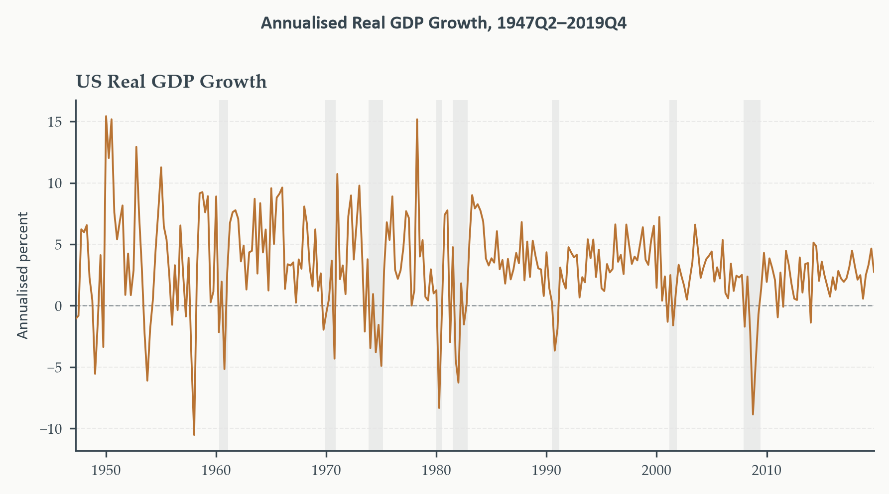
Figure 10.1 makes immediately visible is that the quarterly real GDP growth
rate — the annualised log difference of [`GDPC1`](https://fred.stlouisfed.org/series/GDPC1/) — looks qualitatively different
during those shaded periods than outside them. Outside recessions, growth is
positive, moderately persistent, and clustered around a stable trend. During
recessions, growth turns sharply negative, the volatility increases, and the
series behaves like a different data-generating process altogether.
```{python}
#| label: fig-gdp-growth
#| fig-cap: "Annualised quarterly real GDP growth (log difference × 400),
#| 1947Q2–2019Q4. NBER recessions shaded in grey. The series clusters
#| around a positive mean during expansions and turns sharply negative
#| during recessions. A single linear model treats all observations as
#| draws from the same distribution — a restriction the data clearly
#| challenge."
fig, ax = plt.subplots(figsize=(6, 3.2))

ax.plot(growth_index, growth, color=EO_COPPER, lw=0.9, zorder=3)
ax.axhline(0, color=EO_CHARCOAL, lw=0.6, ls="--", alpha=0.5)

shade_recessions(ax, start=SAMPLE_START, end=SAMPLE_END)
ax.set_xlim(growth_index[0], growth_index[-1])
ax.set_ylabel("Annualised percent")
ax.set_title("US Real GDP Growth")
eo_style_ax(ax)
eo_suptitle(fig, "Annualised Real GDP Growth, 1947Q2–2019Q4")
fig.tight_layout()
plt.show()
```
*Annualised quarterly real GDP growth, 1947Q2–2019Q4. The series clusters
around a positive trend during expansions but turns sharply negative during
recessions (shaded). The dominant feature is the shift in the conditional
mean — a gap of more than 5 pp between the two phases. A model with a
single fixed mean is a poor description of both simultaneously.*
### The Distribution of Growth Is Not a Single Bell Curve
A useful diagnostic is to examine the unconditional distribution of GDP
growth — the histogram of all quarterly observations pooled together. If
a single fixed-parameter model were adequate, this histogram should look
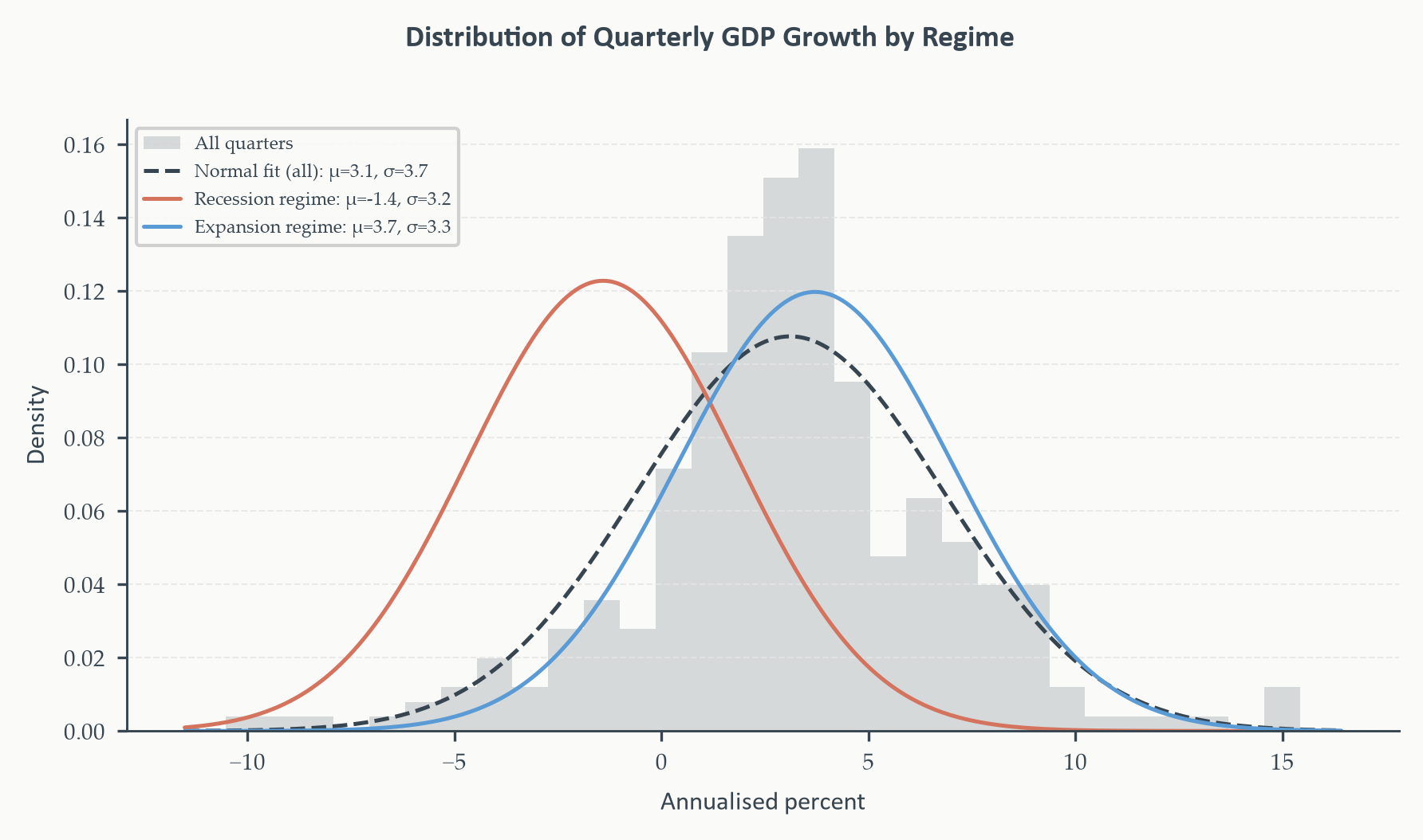
roughly bell-shaped, perhaps slightly skewed but unimodal. Figure 10.2 shows
what the data actually produce.
```{python}
#| label: fig-growth-hist
#| fig-cap: "Histogram of annualised quarterly GDP growth, 1947Q2–2019Q4,
#| with a fitted normal distribution (dashed) and separate normal fits
#| for recession quarters (terracotta) and expansion quarters (sky blue).
#| The pooled distribution is left-skewed and poorly centred — the single
#| normal is pulled between two subpopulations with means 5 pp apart.
#| The regime-specific normals fit their respective subsamples well,
#| motivating a two-component mixture."
# Identify recession quarters
recession_mask = np.zeros(len(gdp), dtype=bool)
for rec_start, rec_end in RECESSIONS:
    s, e = pd.Timestamp(rec_start), pd.Timestamp(rec_end)
    recession_mask |= ((gdp.index >= s) & (gdp.index <= e))

growth_rec = growth[recession_mask]
growth_exp = growth[~recession_mask]

fig, ax = plt.subplots(figsize=(6, 3.4))

# Full-sample histogram
ax.hist(growth, bins=30, density=True,
        color=EO_CHARCOAL, alpha=0.18, label="All quarters")

# Fitted normal to full sample
x_grid = np.linspace(growth.min() - 1, growth.max() + 1, 300)
mu_all, sig_all = growth.mean(), growth.std()
ax.plot(x_grid, stats.norm.pdf(x_grid, mu_all, sig_all),
        color=EO_CHARCOAL, lw=1.2, ls="--", label=f"Normal fit (all): μ={mu_all:.1f}, σ={sig_all:.1f}")

# Regime-specific normals
mu_rec, sig_rec = growth_rec.mean(), growth_rec.std()
mu_exp, sig_exp = growth_exp.mean(), growth_exp.std()
ax.plot(x_grid, stats.norm.pdf(x_grid, mu_rec, sig_rec),
        color=EO_TERRACOTTA, lw=1.2,
        label=f"Recession regime: μ={mu_rec:.1f}, σ={sig_rec:.1f}")
ax.plot(x_grid, stats.norm.pdf(x_grid, mu_exp, sig_exp),
        color=EO_SKYBLUE, lw=1.2,
        label=f"Expansion regime: μ={mu_exp:.1f}, σ={sig_exp:.1f}")

ax.set_xlabel("Annualised percent")
ax.set_ylabel("Density")
ax.legend(fontsize=5.5, loc="upper left")
eo_style_ax(ax)
eo_suptitle(fig, "Distribution of Quarterly GDP Growth by Regime")
fig.tight_layout()
plt.show()
```
*Histogram of quarterly GDP growth with three normal fits superimposed. The
single pooled normal (dashed) understates the left tail and produces a poor
fit in both modes. The recession-specific normal (terracotta) fits the
contraction observations well; the expansion-specific normal (sky blue) fits
the growth observations well. The data are better described as a mixture of
two distributions than as a single one.*
The visual case is reinforced by a simple numerical summary. Using NBER dates
to classify each quarter:
```{python}
#| label: tbl-regime-summary
#| code-summary: "Show code"
n_rec = recession_mask.sum()
n_exp = (~recession_mask).sum()
pct_rec = 100 * n_rec / len(gdp)

print(f"{'─'*58}")
print(f"  GDP Growth Summary Statistics by Business Cycle Phase")
print(f"  1947Q2–2019Q4  (N = {len(gdp)} quarters)")
print(f"{'─'*58}")
print(f"  {'Statistic':<22} {'Expansions':>12} {'Recessions':>12}")
print(f"  {'─'*52}")
print(f"  {'Observations':<22} {n_exp:>12d} {n_rec:>12d}")
print(f"  {'Share of sample':<22} {100-pct_rec:>11.1f}% {pct_rec:>11.1f}%")
print(f"  {'Mean (ann. %)':<22} {mu_exp:>12.2f} {mu_rec:>12.2f}")
print(f"  {'Std dev (ann. %)':<22} {sig_exp:>12.2f} {sig_rec:>12.2f}")
print(f"  {'Minimum':<22} {growth_exp.min():>12.2f} {growth_rec.min():>12.2f}")
print(f"  {'Maximum':<22} {growth_exp.max():>12.2f} {growth_rec.max():>12.2f}")
print(f"{'─'*58}")
print(f"  Note: recession classification from NBER Business Cycle Dating")
print(f"  Committee. Recession quarters are those falling within an")
print(f"  official contraction as defined by NBER peak-to-trough dates.")
print(f"{'─'*58}")
```
*GDP growth summary statistics by NBER business cycle phase. The mean growth
rate in expansion quarters is 3.71 pp; in recession quarters it is −1.41 pp —
a gap of 5.1 pp. The standard deviations are nearly identical (3.33 vs. 3.25),
so the dominant difference between regimes is the mean, not the variance. Any
model that imposes the same mean across both phases is misspecified by
construction.*
The mean gap between the two phases is the decisive finding: 5.1 pp is large
both economically and statistically. The standard deviations are nearly
identical across regimes — 3.33 pp in expansions and 3.25 pp in recessions —
so this is primarily a story about mean switching, not variance switching.
A model that pools the two regimes is not a harmless simplification — it
produces a mean that belongs to neither phase. The Markov-switching framework
provides the principled resolution: let the mean be regime-specific, treat the
regime as a latent state that the data can inform, and let the estimation
determine whether variance switching adds enough to justify the extra
parameters.
### What a Regime-Switching Model Does Differently
Before we write down a single equation, it is worth stating plainly what the
Markov-switching approach contributes and what it costs.
What it contributes: the model explicitly allows the data-generating process
to be different in different phases of the business cycle. The expansion mean,
the recession mean, the expansion variance, and the recession variance are all
estimated from the data. The model also estimates the probability of staying in
each regime and the probability of switching — parameters that have direct
economic content as measures of cycle duration.
What it costs: the parameters of the model are no longer identified by a
simple OLS regression. The regime is unobserved, so estimation requires
integrating over all possible regime paths — a task handled by the Hamilton
filter. The model is nonlinear: the observed GDP growth is a mixture of two
(or more) Gaussians with mixture weights that depend on the unobserved state.
And the number of regimes is a modelling choice that must be made on economic
grounds before estimation, since standard likelihood-ratio tests do not have
their usual distributions when comparing models with different numbers of
regimes.
::: {.callout-warning icon=false}
## Testing for the Number of Regimes
Standard regularity conditions for likelihood-ratio tests fail when comparing
a model with $M$ regimes against one with $M-1$ regimes. Under the null
hypothesis of $M-1$ regimes, the parameters specific to the $M$-th regime are
unidentified, and the transition probabilities lie on the boundary of their
parameter space. As a result, the LR statistic does not follow a $\chi^2$
distribution. In practice, the number of regimes is typically chosen on
economic grounds (two regimes for the business cycle is the canonical
choice) and validated by the interpretability of the estimated regimes rather
than by a formal test. Information criteria such as AIC and BIC can be used
for model comparison after estimation, though their theoretical properties in
this context are less well established than in the linear case.
:::
These costs are real but manageable. [Hamilton's (1989)](https://doi.org/10.2307/1912559) two-state model has
been applied to US GDP growth for more than three decades, and its ability to
identify recessions without using NBER dates has made it one of the most
influential papers in macroeconometrics. We build it from scratch in the next
section.
## The Two-State Markov-Switching Model {#sec-msmodel}
### The Hidden State
At the heart of every Markov-switching model is a simple idea: there exists
an unobserved state variable $s_t$ that determines which regime the economy
is in at time $t$. In the two-state model, this variable takes only two values:
$$
s_t \in \{0, 1\}
\tag{10.1}
$$
where, following convention, $s_t = 0$ denotes the expansion regime and
$s_t = 1$ denotes the recession regime. The state is not directly observed —
we never see $s_t$ in the data, only the GDP growth series $y_t$ that it
influences. Inferring $s_t$ from $y_t$ is the filtering problem that occupies
Section 10.3.
### The Transition Probability Matrix
The state $s_t$ evolves over time. We assume it follows a first-order Markov
chain: the probability that the economy is in regime $j$ next period depends
only on which regime it is in this period, not on the full history of past
states. This gives us four transition probabilities:
$$
\begin{aligned}
p_{00} &= \Pr(s_t = 0 \mid s_{t-1} = 0) \\
p_{10} &= \Pr(s_t = 1 \mid s_{t-1} = 0) \\
p_{01} &= \Pr(s_t = 0 \mid s_{t-1} = 1) \\
p_{11} &= \Pr(s_t = 1 \mid s_{t-1} = 1)
\end{aligned}
$$
Since the state must go somewhere — the economy is always in one regime or
the other — the probabilities in each row must sum to one:
$$
p_{00} + p_{10} = 1 \qquad p_{01} + p_{11} = 1
\tag{10.2}
$$
We collect these into the transition probability matrix $P$:
$$
P = \begin{pmatrix} p_{00} & p_{10} \\ p_{01} & p_{11} \end{pmatrix}
\tag{10.3}
$$
where entry $(i, j)$ gives the probability of transitioning from state $i$
to state $j$. Because of the two sum-to-one constraints, only two parameters
are free: the probability of staying in expansion $p_{00}$ and the probability
of staying in recession $p_{11}$. These are the core parameters of the
Markov chain.
::: {.callout-note}
## Definition 10.1 — First-Order Markov Chain
A discrete-valued stochastic process $\{s_t\}$ is a **first-order Markov
chain** if, for all $t$ and all possible state histories,
$$
\Pr(s_t = j \mid s_{t-1}, s_{t-2}, \ldots) = \Pr(s_t = j \mid s_{t-1})
$$
The probability of being in state $j$ at time $t$ depends only on the state
at $t-1$, not on earlier history. The two-state version requires only the
transition matrix $P$ to characterise all dynamics of the chain.
:::
### Reading the Transition Matrix Economically
The transition probabilities have direct economic interpretations that make
them more than statistical parameters. Consider $p_{00}$, the probability
of remaining in the expansion state from one quarter to the next. If this
parameter is estimated to be $0.94$, then conditional on being in an
expansion today, there is a 94% chance of still being in expansion next
quarter. The implied average duration of an expansion is:
$$
\mathbb{E}[\text{expansion duration}] = \frac{1}{1 - p_{00}} = \frac{1}{0.06} \approx 17 \text{ quarters}
\tag{10.4}
$$
Similarly, if $p_{11} = 0.75$, the average recession lasts:
$$
\mathbb{E}[\text{recession duration}] = \frac{1}{1 - p_{11}} = \frac{1}{0.25} = 4 \text{ quarters}
\tag{10.5}
$$
These duration formulas follow from the geometric distribution: if the
probability of leaving a state is constant at $1 - p_{ii}$ each period,
the number of periods spent in that state before switching follows a geometric
distribution with mean $1/(1-p_{ii})$. Postwar US business cycle durations —
expansions lasting many years, recessions lasting roughly a year — are
consistent with transition probabilities in this ballpark, which is part of
why Hamilton's model fits the data well.
### The Ergodic Distribution
Over the long run, the fraction of time the economy spends in each regime
converges to a fixed distribution — the ergodic (or stationary) distribution
of the Markov chain. Think of it as the long-run answer to the question: "if
we ran this economy for a thousand quarters, what fraction of them would be
recessions?" That fraction is pinned down entirely by how sticky each regime
is — how rarely the economy leaves expansion, and how rarely it leaves
recession — not by where it started. A chain that almost never leaves
expansion ($p_{00}$ close to 1) will spend most of its time there regardless
of initial conditions; a chain that switches frequently will divide its time
more evenly. The ergodic distribution formalises this intuition.
Let $\pi_0$ and $\pi_1 = 1 - \pi_0$ denote the ergodic probabilities of
being in the expansion and recession states. We find them by imposing a
fixed-point condition: if the distribution is truly stationary, then the
probability of being in expansion this period must be the same as next period.
That self-replicating requirement gives:
$$
\pi_0 = \pi_0 \, p_{00} + \pi_1 \, p_{01}
\tag{10.6}
$$
Both sides carry $\pi_0$ because we are solving for the value of $\pi_0$ that
is left unchanged by one step of the transition matrix — the right side says
"we arrive in expansion either by staying from expansion (probability
$\pi_0 p_{00}$) or by switching from recession (probability $\pi_1 p_{01}$)",
and the equation asks for that arrival probability to equal the departure
probability $\pi_0$.
Substituting $\pi_1 = 1 - \pi_0$ and solving:
$$
\begin{aligned}
\pi_0 &= \pi_0 \, p_{00} + (1 - \pi_0) \, p_{01} \\
\pi_0 (1 - p_{00} + p_{01}) &= p_{01} \\
\pi_0 &= \frac{p_{01}}{1 - p_{00} + p_{01}} = \frac{1 - p_{11}}{(1 - p_{00}) + (1 - p_{11})}
\end{aligned}
$$
which gives the compact result:
$$
\pi_0 = \frac{1 - p_{11}}{2 - p_{00} - p_{11}}, \qquad \pi_1 = \frac{1 - p_{00}}{2 - p_{00} - p_{11}}
\tag{10.7}
$$
**Numerical example.** Suppose $p_{00} = 0.94$ and $p_{11} = 0.75$. Then:
$$
\pi_0 = \frac{1 - 0.75}{(1 - 0.94) + (1 - 0.75)} = \frac{0.25}{0.06 + 0.25} = \frac{0.25}{0.31} \approx 0.81
$$
The economy is in expansion 81% of the time in the long run — consistent with
the NBER classification that roughly 15–20% of postwar quarters are
recessionary. Note that this result falls directly out of the two transition
probabilities: we did not need to specify anything about GDP growth itself.
```{python}
#| label: ergodic-example
#| code-summary: "Show code"
# Numerical illustration of ergodic distribution
p00_ex = 0.94
p11_ex = 0.75
p10_ex = 1 - p00_ex   # prob of leaving expansion
p01_ex = 1 - p11_ex   # prob of leaving recession

pi0 = p01_ex / (p10_ex + p01_ex)
pi1 = 1 - pi0

dur_exp = 1 / p10_ex
dur_rec = 1 / p01_ex

print(f"{'─'*52}")
print(f"  Ergodic Distribution — Numerical Example")
print(f"{'─'*52}")
print(f"  Transition probabilities:")
print(f"    p₀₀ (stay in expansion) = {p00_ex:.2f}")
print(f"    p₁₁ (stay in recession) = {p11_ex:.2f}")
print(f"")
print(f"  Ergodic probabilities:")
print(f"    π₀ (long-run expansion share) = {pi0:.3f}  ({100*pi0:.1f}%)")
print(f"    π₁ (long-run recession share) = {pi1:.3f}  ({100*pi1:.1f}%)")
print(f"")
print(f"  Implied average durations:")
print(f"    Expansion: 1/(1−p₀₀) = {dur_exp:.1f} quarters ≈ {dur_exp/4:.1f} years")
print(f"    Recession: 1/(1−p₁₁) = {dur_rec:.1f} quarters ≈ {dur_rec/4:.1f} years")
print(f"{'─'*52}")
```
*Ergodic distribution and implied durations for the illustrative transition
matrix. With $p_{00} = 0.94$ and $p_{11} = 0.75$, the economy spends about
81% of its time in expansion and 19% in recession. The average expansion lasts
roughly 17 quarters; the average recession lasts 4 quarters. Both figures are
broadly consistent with postwar NBER cycle chronology.*
### The MS-AR Mean Equation
With the Markov chain in place, we can write down the model for GDP growth.
In the simplest specification — mean-switching only, no AR dynamics — the
conditional mean switches with the regime while the variance stays fixed:
$$
y_t = \mu_{s_t} + \varepsilon_t, \qquad \varepsilon_t \sim \mathcal{N}(0, \sigma^2)
\tag{10.8}
$$
where $\mu_0$ is the mean growth rate in expansion and $\mu_1$ is the mean
growth rate in recession. This already imposes a mixture distribution on $y_t$:
in any quarter, the observed growth rate is drawn from $\mathcal{N}(\mu_0, \sigma^2)$
with probability $\pi_0$ or from $\mathcal{N}(\mu_1, \sigma^2)$ with probability
$\pi_1$, with the specific draw determined by the hidden state.
Hamilton's original (1989) model adds AR dynamics and allows the variance to
switch as well. We adopt the variance-switching MS-AR(2) specification as the
working model for this chapter:
$$
y_t = \mu_{s_t} + \phi_1(y_{t-1} - \mu_{s_{t-1}}) + \phi_2(y_{t-2} - \mu_{s_{t-2}}) + \varepsilon_t
\tag{10.9}
$$
$$
\varepsilon_t \sim \mathcal{N}(0, \sigma_{s_t}^2)
\tag{10.10}
$$
Equation (10.9) expresses GDP growth as a regime-specific mean plus
autoregressive corrections based on how far the two preceding quarters
deviated from their own regime means. Equation (10.10) allows the innovation
variance to differ across regimes. The AR coefficients $\phi_1$ and $\phi_2$
are constrained to be the same across regimes in this specification; allowing
them to switch as well is a natural extension but adds parameters quickly.
::: {.callout-note}
## Definition 10.2 — MS-AR($k$) Model
A **Markov-switching autoregression of order $k$** specifies:
$$
y_t = \mu_{s_t} + \sum_{j=1}^{k} \phi_j (y_{t-j} - \mu_{s_{t-j}}) + \varepsilon_t,
\qquad \varepsilon_t \sim \mathcal{N}(0, \sigma_{s_t}^2)
$$
where $s_t \in \{0, 1, \ldots, M-1\}$ follows a first-order Markov chain
with transition matrix $P$. The parameters $\mu_m$, $\sigma_m^2$ are
regime-specific; the AR coefficients $\phi_j$ are shared across regimes.
The full parameter vector is $\theta = (\mu_0, \mu_1, \sigma_0^2, \sigma_1^2,
\phi_1, \ldots, \phi_k, p_{00}, p_{11})$.
:::
It is worth pausing on what makes equation (10.9) nonlinear. The term
$\mu_{s_{t-j}}$ is the regime-specific mean evaluated at the regime in period
$t-j$ — not the regime in period $t$. This means the autoregressive correction
depends on which regime applied in earlier periods, which in turn was
unobserved. When we condition on having been in regime $m$ at $t-1$ and regime
$n$ at $t-2$, the conditional distribution of $y_t$ given $s_t = r$ is Gaussian
with a specific mean and variance — but to evaluate the likelihood, we must
sum over all possible past regime combinations. This is what the Hamilton
filter does.
### Mean-Switching vs. Variance-Switching vs. Both
The MS framework is flexible enough to separate mean switching from variance
switching. Table 10.1 summarises the main specifications.
```{python}
#| label: tbl-ms-specs
#| code-summary: "Show code"
print(f"{'─'*70}")
print(f"  Table 10.1 — Markov-Switching Specifications")
print(f"{'─'*70}")
print(f"  {'Specification':<28} {'Mean switches':<16} {'Variance switches':<18} {'Parameters'}")
print(f"  {'─'*64}")
print(f"  {'Mean-switching only':<28} {'Yes':<16} {'No':<18} μ₀, μ₁, σ², p₀₀, p₁₁")
print(f"  {'Variance-switching only':<28} {'No':<16} {'Yes':<18} μ, σ₀², σ₁², p₀₀, p₁₁")
print(f"  {'Mean and variance switching':<28} {'Yes':<16} {'Yes':<18} μ₀, μ₁, σ₀², σ₁², p₀₀, p₁₁")
print(f"  {'MS-AR(k), mean only':<28} {'Yes':<16} {'No':<18} + φ₁,…,φₖ")
print(f"  {'MS-AR(k), mean and var.':<28} {'Yes':<16} {'Yes':<18} + φ₁,…,φₖ")
print(f"{'─'*70}")
print(f"  Note: AR coefficients are constrained equal across regimes in all")
print(f"  specifications above. Allowing φ to switch multiplies the AR")
print(f"  parameter count by the number of regimes M.")
print(f"{'─'*70}")
```
*Main Markov-switching specifications. The mean-switching model is the
simplest and most interpretable: it identifies two levels of average growth.
Variance switching adds a further degree of freedom that may or may not be
supported by the data — in our GDP growth sample, the regime-specific standard
deviations are nearly equal, so the mean-switching specification captures most
of the action. The MS-AR specifications add persistence to the within-regime
dynamics. The working model for this chapter is the **mean-switching** MS-AR(2)
of equations (10.9)–(10.10): common variance, regime-specific means. This follows
Hamilton (1989) and avoids the estimation difficulties that arise when variance
is also free to switch on a sample where recessions are only 12% of quarters.*
For our GDP growth application, the case for mean switching is clear and
strong: the 5.1 pp gap between the expansion mean (3.71%) and the recession
mean (−1.41%) is the dominant feature of the data. The standard deviations are
nearly identical across the two NBER-classified phases, so variance switching
adds little signal but creates an estimation problem — the likelihood surface
has a variance-only local optimum that is numerically easier to find than the
mean-switching solution. The working model for this chapter is therefore
mean-switching with a common variance, following [Hamilton (1989)](https://doi.org/10.2307/1912559) exactly. We
return to variance switching as a modelling choice in Section 10.4.
## The Hamilton Filter {#sec-hamilton}
### The Inference Problem
We now have a model: GDP growth $y_t$ is generated by a regime-specific mean
and variance, with the regime $s_t$ evolving as a hidden Markov chain. The
estimation and forecasting questions both require us to answer the same
underlying question: given what we have observed up to time $t$, what is the
probability that the economy is currently in each regime? More precisely, we
want to compute:
$$
\Pr(s_t = j \mid y_t, y_{t-1}, \ldots, y_1), \qquad j \in \{0, 1\}
\tag{10.11}
$$
This is a filtering problem. The state $s_t$ is hidden; the observations
$y_1, \ldots, y_t$ carry information about it. The Hamilton filter is the
recursive algorithm that extracts that information efficiently, processing
one observation at a time from left to right through the sample.
The filter produces two objects at each date $t$:
- **Filtered probabilities**: $\xi_{t|t} = \Pr(s_t = j \mid y_1, \ldots, y_t)$ —
the probability of being in each regime given all data up to and including
$t$. This is the real-time inference an econometrician could have made
in period $t$.
- **Predicted probabilities**: $\xi_{t|t-1} = \Pr(s_t = j \mid y_1, \ldots, y_{t-1})$ —
the probability of being in each regime given data up to $t-1$, before
observing $y_t$. This is the one-step-ahead forecast of the regime.
A third object — smoothed probabilities — uses the full sample
$y_1, \ldots, y_T$ to infer the regime at each date retrospectively. We
return to this distinction after deriving the filter.
### The Filter Recursion
The filter alternates between two steps at each $t$: a **prediction step**
that uses the transition matrix to project the regime probability forward,
and an **update step** that uses the new observation $y_t$ to revise that
prediction. Both steps are applications of [Bayes' rule](https://en.wikipedia.org/wiki/Bayes%27_theorem).
**Step 1 — Prediction.** Given the filtered probability $\xi_{t-1|t-1}$ at
the end of period $t-1$, we predict the regime probability at period $t$
before observing $y_t$:
$$
\xi_{t|t-1} = P' \, \xi_{t-1|t-1}
\tag{10.12}
$$
where $P'$ is the transpose of the transition matrix and $\xi_{t-1|t-1}$ is
the column vector $(\Pr(s_{t-1}=0 \mid \mathcal{F}_{t-1}),\, \Pr(s_{t-1}=1
\mid \mathcal{F}_{t-1}))'$. Written out for the two-state case:
$$
\begin{aligned}
\Pr(s_t = 0 \mid \mathcal{F}_{t-1}) &= p_{00}\, \Pr(s_{t-1}=0 \mid \mathcal{F}_{t-1})
+ p_{01}\, \Pr(s_{t-1}=1 \mid \mathcal{F}_{t-1}) \\
\Pr(s_t = 1 \mid \mathcal{F}_{t-1}) &= p_{10}\, \Pr(s_{t-1}=0 \mid \mathcal{F}_{t-1})
+ p_{11}\, \Pr(s_{t-1}=1 \mid \mathcal{F}_{t-1})
\end{aligned}
$$
The predicted probability of being in expansion tomorrow is the probability
of being in expansion today and staying, plus the probability of being in
recession today and switching. No observation of $y_t$ has been used yet.
**Step 2 — Update.** When $y_t$ arrives, we use it to revise the predicted
regime probabilities via [Bayes' rule](https://en.wikipedia.org/wiki/Bayes%27_theorem). The conditional density of $y_t$ given
regime $j$ and the past is:
$$
f(y_t \mid s_t = j,\, \mathcal{F}_{t-1}) = \frac{1}{\sqrt{2\pi\sigma_j^2}}
\exp\!\left(-\frac{(y_t - \mu_j^*)^2}{2\sigma_j^2}\right)
\tag{10.13}
$$
where $\mu_j^*$ is the regime-$j$ conditional mean of $y_t$ given past data
(from the AR terms in equation (10.9)). Applying [Bayes' rule](https://en.wikipedia.org/wiki/Bayes%27_theorem):
$$
\Pr(s_t = j \mid \mathcal{F}_t) = \frac{f(y_t \mid s_t = j,\, \mathcal{F}_{t-1})
\cdot \Pr(s_t = j \mid \mathcal{F}_{t-1})}{\sum_{m=0}^{1} f(y_t \mid s_t = m,\,
\mathcal{F}_{t-1}) \cdot \Pr(s_t = m \mid \mathcal{F}_{t-1})}
\tag{10.14}
$$
In words: the updated probability that we are in regime $j$ is proportional
to how likely $y_t$ was under regime $j$ (the likelihood) times how likely
we thought regime $j$ was before seeing $y_t$ (the prior). The denominator
normalises so the two probabilities sum to one. This denominator is also the
marginal density of $y_t$ given past data — summing it across $t$ gives the
log-likelihood used for estimation.
::: {.callout-note}
## Definition 10.3 — The Hamilton Filter
Given initial probabilities $\xi_{1|0}$ (typically set to the ergodic
distribution), the **Hamilton filter** iterates for $t = 1, \ldots, T$:
1. **Predict**: $\xi_{t|t-1} = P' \xi_{t-1|t-1}$
2. **Evaluate**: compute $\eta_t = (f(y_t \mid s_t=0,\mathcal{F}_{t-1}),\;
f(y_t \mid s_t=1,\mathcal{F}_{t-1}))'$
3. **Update**: $\xi_{t|t} = (\eta_t \odot \xi_{t|t-1})\, /\, (\mathbf{1}'\,
(\eta_t \odot \xi_{t|t-1}))$
where $\odot$ denotes element-wise multiplication and $\mathbf{1}'
(\eta_t \odot \xi_{t|t-1})$ is the normalising constant. The log-likelihood
is $\ell(\theta) = \sum_{t=1}^T \log\bigl(\mathbf{1}'(\eta_t \odot
\xi_{t|t-1})\bigr)$.
:::
### A Numerical Example
Before implementing the filter on real data, it is worth tracing through two
periods by hand to make the mechanics concrete. Suppose we have a mean-switching
model with $\mu_0 = 3$, $\mu_1 = -2$, $\sigma^2 = 4$ (common variance),
$p_{00} = 0.9$, $p_{11} = 0.7$. The ergodic distribution from equation (10.7)
gives $\pi_0 = 0.75$, $\pi_1 = 0.25$, which we use as initial probabilities.
**Period $t = 1$:** Suppose $y_1 = 4.2$ (a strong expansion quarter).
Predicted probabilities (from the ergodic initialisation):
$\Pr(s_1 = 0 \mid \mathcal{F}_0) = 0.75$,
$\Pr(s_1 = 1 \mid \mathcal{F}_0) = 0.25$.
Conditional densities under each regime:
$$
\begin{aligned}
f(y_1 \mid s_1 = 0) &= \phi\!\left(\frac{4.2 - 3}{\sqrt{4}}\right) = \phi(0.60) \approx 0.333 \\
f(y_1 \mid s_1 = 1) &= \phi\!\left(\frac{4.2 - (-2)}{\sqrt{4}}\right) = \phi(3.10) \approx 0.003
\end{aligned}
$$
where $\phi(\cdot)$ is the standard normal density. The observation
$y_1 = 4.2$ is far more consistent with the expansion regime. Applying
the update step:
$$
\Pr(s_1 = 0 \mid y_1) = \frac{0.333 \times 0.75}{0.333 \times 0.75 + 0.003 \times 0.25}
= \frac{0.250}{0.251} \approx 0.996
$$
After observing a growth rate of 4.2%, the filter assigns a 99.6% probability
to the expansion regime.
**Period $t = 2$:** Suppose $y_2 = -3.8$ (a contraction).
Prediction step: carry forward the $t=1$ filtered probability through the
transition matrix:
$$
\begin{aligned}
\Pr(s_2 = 0 \mid y_1) &= 0.9 \times 0.996 + 0.3 \times 0.004 \approx 0.897 \\
\Pr(s_2 = 1 \mid y_1) &= 0.1 \times 0.996 + 0.7 \times 0.004 \approx 0.103
\end{aligned}
$$
Even before seeing $y_2$, the high persistence of expansions keeps the
predicted expansion probability at 89.7%. Now the observation $y_2 = -3.8$
arrives — a sharp contraction. The conditional densities are:
$$
\begin{aligned}
f(y_2 \mid s_2 = 0) &= \phi\!\left(\frac{-3.8 - 3}{2}\right) = \phi(-3.40) \approx 0.001 \\
f(y_2 \mid s_2 = 1) &= \phi\!\left(\frac{-3.8 - (-2)}{2}\right) = \phi(-0.90) \approx 0.266
\end{aligned}
$$
Updating:
$$
\Pr(s_2 = 0 \mid y_1, y_2) = \frac{0.001 \times 0.897}{0.001 \times 0.897 + 0.266 \times 0.103}
= \frac{0.001}{0.028} \approx 0.032
$$
One quarter of sharply negative growth has driven the expansion probability
from 89.7% down to 3.2%. This is the filter doing its job: incorporating the
new observation rapidly and decisively when it is highly informative.
```{python}
#| label: hamilton-numerical
#| code-summary: "Show code"
# ── Numerical Hamilton filter example ─────────────────────────────────────────
mu0, mu1 = 3.0, -2.0
sigma2    = 4.0
p00_n, p11_n = 0.90, 0.70
p01_n = 1 - p11_n
p10_n = 1 - p00_n

# Ergodic initialisation
pi0_n = p01_n / (p10_n + p01_n)
pi1_n = 1 - pi0_n

observations = [4.2, -3.8]
xi_pred = np.array([pi0_n, pi1_n])   # initial predicted probabilities

print(f"{'─'*58}")
print(f"  Hamilton Filter — Two-Period Numerical Example")
print(f"  μ₀={mu0}, μ₁={mu1}, σ²={sigma2}, p₀₀={p00_n}, p₁₁={p11_n}")
print(f"  Initial (ergodic): π₀={pi0_n:.3f}, π₁={pi1_n:.3f}")
print(f"{'─'*58}")

P_n = np.array([[p00_n, p10_n],
                [p01_n, p11_n]])

for t, y in enumerate(observations, start=1):
    # Conditional densities
    eta = np.array([stats.norm.pdf(y, mu0, np.sqrt(sigma2)),
                    stats.norm.pdf(y, mu1, np.sqrt(sigma2))])

    # Normalising constant (marginal density of y_t)
    denom = eta @ xi_pred

    # Updated (filtered) probabilities
    xi_filt = (eta * xi_pred) / denom

    print(f"\n  t = {t},  y_t = {y}")
    print(f"  {'─'*50}")
    print(f"  Predicted :  Pr(s={0}│past) = {xi_pred[0]:.3f},"
          f"  Pr(s={1}│past) = {xi_pred[1]:.3f}")
    print(f"  Densities :  f(y│s=0) = {eta[0]:.4f},  f(y│s=1) = {eta[1]:.4f}")
    print(f"  Filtered  :  Pr(s={0}│data) = {xi_filt[0]:.3f},"
          f"  Pr(s={1}│data) = {xi_filt[1]:.3f}")

    # Predict forward for next period
    xi_pred = P_n.T @ xi_filt

print(f"\n{'─'*58}")
```
*Hamilton filter traced through two periods. At $t=1$ the observation $y_1 = 4.2$
is highly informative about the expansion regime: the filtered expansion
probability rises to 99.6%. At $t=2$ the observation $y_2 = -3.8$ is strongly
consistent with recession: the expansion probability collapses to 3.2% despite
entering the period at 89.7%. The filter updates sharply when observations are
far from one regime mean and close to the other.*
### Filtered vs. Smoothed Probabilities
The Hamilton filter produces **filtered probabilities** $\xi_{t|t}$ — the
best estimate of the current regime using only data available through period
$t$. These are the probabilities a real-time forecaster could have computed.
They are causal: no future observation influences $\xi_{t|t}$.
**Smoothed probabilities** $\xi_{t|T}$ use the full sample $y_1, \ldots, y_T$
to form a retrospective estimate of the regime at each date $t \leq T$. The
smoothing algorithm runs the filter forward from $t=1$ to $T$, then passes
backward from $T$ to $1$, propagating information from future observations
back through the transition structure. The [Kim (1994])(https://www.sciencedirect.com/science/article/abs/pii/0304407694900361) smoother is the standard
implementation:
$$
\xi_{t|T} = \xi_{t|t} \odot \left[ P \left(\xi_{t+1|T} \,/\, \xi_{t+1|t}\right) \right]
\tag{10.15}
$$
where the division is element-wise and $P$ is the transition matrix. Smoothed
probabilities are sharper — they assign more decisive regime classifications
— because they incorporate evidence that a recession began or ended near date
$t$ even if that evidence only arrived in later periods.
::: {.callout-warning icon=false}
## Filtered vs. Smoothed: Which to Use
Use **filtered probabilities** when the question is about real-time inference:
"what would an econometrician have known in period $t$?" This is the relevant
object for forecasting exercises and for replicating Hamilton's original
real-time recession detection.
Use **smoothed probabilities** when the question is about historical
classification: "given everything we now know, which quarters were most likely
recessions?" Smoothed probabilities are appropriate for comparing the
model's regime estimates against NBER dates, since the NBER's own
classifications are also retrospective. Using smoothed probabilities for
real-time forecasting evaluation would introduce look-ahead bias.
:::
### Connection to the Kalman Filter
The Hamilton filter and the Kalman filter of Chapter 11 solve the same
underlying problem — extracting a hidden state from a noisy observation
sequence — using the same prediction-correction logic. Both begin with a
prior distribution over the hidden state, compute the likelihood of the
observation under that prior, and update to a posterior. Both then project
the posterior forward through the state transition equation to form the
prior for the next period.
The critical difference is the state space. In the Hamilton filter, the
state $s_t$ is discrete — it takes two values — so the prior and posterior
are probability vectors of dimension $M$ and the "densities" are Gaussian
mixtures. In the Kalman filter, the state $\alpha_t$ is continuous and
Gaussian, so the prior and posterior are fully described by a mean vector
and a covariance matrix, and the update equations are linear. The Kalman
filter is, in a precise sense, the Gaussian-state analogue of the Hamilton
filter. Recognising this parallel will make Chapter 11 immediately
navigable: the predict step, the update step, and the smoother all have
direct counterparts.
## Estimation and Empirical Results {#sec-estimation}
### Maximum Likelihood via the Hamilton Filter
The Hamilton filter delivers more than regime probabilities — it also delivers
the log-likelihood of the observed data under any parameter vector $\theta$.
At each step $t$, the normalising constant in the update equation (10.14) is
the marginal density of $y_t$ given past data:
$$
f(y_t \mid \mathcal{F}_{t-1};\, \theta) = \sum_{j=0}^{1}
f(y_t \mid s_t = j,\, \mathcal{F}_{t-1};\, \theta)\cdot
\Pr(s_t = j \mid \mathcal{F}_{t-1};\, \theta)
\tag{10.16}
$$
Summing log-densities across $t$ gives the full-sample log-likelihood:
$$
\ell(\theta) = \sum_{t=1}^{T} \log f(y_t \mid \mathcal{F}_{t-1};\, \theta)
\tag{10.17}
$$
MLE proceeds by maximising $\ell(\theta)$ over $\theta = (\mu_0, \mu_1,
\sigma_0^2, \sigma_1^2, \phi_1, \phi_2, p_{00}, p_{11})$. Each evaluation of
the objective function requires running the full Hamilton filter — $T$
prediction-update cycles — which makes the likelihood expensive relative to
OLS but tractable for the sample sizes typical in macroeconomics. Standard
numerical optimisers (BFGS, Nelder-Mead) are used in practice; `statsmodels`
wraps this for the two-state MS-AR case.
::: {.callout-warning icon=false}
## Identification and Labelling
The two regimes are interchangeable in the likelihood: swapping all
$j=0$ parameters with all $j=1$ parameters produces an identical value of
$\ell(\theta)$. This labelling indeterminacy means the likelihood surface
has two symmetric regions, and a numerical optimizer may converge to either.
The practical consequence is significant: without guidance, `statsmodels`
can produce a solution in which both regime means are positive — a
variance-only split rather than the economically meaningful mean-switching
solution. The remedy is to supply starting values that encode the economic
prior: the expansion regime has a positive mean near trend growth, and the
recession regime has a negative mean. The estimation code below does this
explicitly. Always verify after estimation that regime 0 has the higher mean
and that the implied ergodic recession share is plausible (roughly 10–20%
for postwar US data).
:::
### Fitting the MS-AR(2) to GDP Growth
We estimate the **mean-switching** MS-AR(2) on annualised quarterly GDP
growth, 1947Q2–2019Q4. Section 10.1 already showed that the NBER-classified
regime standard deviations are nearly identical (3.33 vs. 3.25 pp), so the
mean difference is the dominant feature of the data. Allowing variance to
switch freely creates a practical estimation problem: with only 12% of quarters
in recession, the optimizer tends to find a variance-only split — two
clusters both centred near positive growth, distinguished only by dispersion
— rather than the economically meaningful contraction/expansion separation.
Hamilton’s (1989) original specification was mean-switching only, for exactly
this reason. We follow suit and comment on variance switching at the end of
this section.
```{python}
#| label: ms-estimation
#| code-summary: "Show code"
from statsmodels.tsa.regime_switching.markov_autoregression import MarkovAutoregression

# ── Estimate MS-AR(2): mean-switching only, common variance ──────────────────
# Parameter order: [p[0->0], p[1->0], const[0], const[1], sigma2, ar.L1, ar.L2]
# Mean-switching only (switching_variance=False) follows Hamilton (1989) and
# avoids the variance-only local optimum that afflicts the unrestricted model
# on this sample (NBER recessions = only 12% of quarters).
start_params = np.array([
    0.95,   # p[0->0]: expansion is very persistent
    0.20,   # p[1->0]: recession exits with ~20% probability per quarter
    3.5,    # const[0]: expansion mean ≈ 3.5%
   -1.5,    # const[1]: recession mean ≈ -1.5%
   10.0,    # sigma2: common variance
    0.25,   # ar.L1
    0.10,   # ar.L2
])

ms_model = MarkovAutoregression(
    gdp["GDP Growth"],
    k_regimes=2,
    order=2,
    switching_ar=False,        # AR coefficients common across regimes
    switching_variance=False   # common variance — mean-switching only
)

ms_result = ms_model.fit(start_params=start_params, disp=False)

# ── Ensure regime 0 = expansion (high mean) ───────────────────────────────────
if ms_result.params["const[0]"] < ms_result.params["const[1]"]:
    sp2 = start_params.copy()
    sp2[0], sp2[1] = start_params[1], start_params[0]
    sp2[2], sp2[3] = start_params[3], start_params[2]
    ms_result = ms_model.fit(start_params=sp2, disp=False)

# ── Extract parameters ─────────────────────────────────────────────────────────
mu_hat  = [ms_result.params[f"const[{j}]"] for j in range(2)]
sig_hat = [np.sqrt(ms_result.params["sigma2"])] * 2   # common variance

# Transition probabilities
# statsmodels stores p[i->j] = prob of moving FROM regime i TO regime j
p00_hat = ms_result.params["p[0->0]"]   # stay in expansion
p01_hat = ms_result.params["p[1->0]"]   # leave recession → expansion
p10_hat = 1 - p00_hat                   # leave expansion → recession
p11_hat = 1 - p01_hat                   # stay in recession

# AR coefficients
phi1_hat = ms_result.params["ar.L1"]
phi2_hat = ms_result.params["ar.L2"]

# Ergodic probabilities from estimated transition matrix
pi0_hat = p01_hat / (p10_hat + p01_hat)
pi1_hat = 1 - pi0_hat

# Implied durations
dur_exp_hat = 1 / p10_hat
dur_rec_hat = 1 / p01_hat

# Standard errors
bse = ms_result.bse

print(f"{'─'*62}")
print(f"  MS-AR(2) — GDP Growth, 1947Q2–2019Q4")
print(f"  Mean-switching only (common variance); AR coefficients common")
print(f"{'─'*62}")
print(f"\n  Regime parameters")
print(f"  {'─'*56}")
print(f"  {'Parameter':<28} {'Regime 0 (Expansion)':>16} {'Regime 1 (Recession)':>16}")
print(f"  {'─'*56}")
se_mu0  = f"({bse['const[0]']:.3f})"
se_mu1  = f"({bse['const[1]']:.3f})"
se_phi1 = f"({bse['ar.L1']:.3f})"
se_phi2 = f"({bse['ar.L2']:.3f})"

print(f"  {'Mean μ':<28} {mu_hat[0]:>16.3f} {mu_hat[1]:>16.3f}")
print(f"  {'':28} {se_mu0:>16} {se_mu1:>16}")
print(f"  {'Std dev σ (common)':<28} {sig_hat[0]:>16.3f} {'(common)':>16}")
print(f"\n  AR dynamics (common across regimes)")
print(f"  {'─'*56}")
print(f"  {'φ₁':<28} {phi1_hat:>16.3f}")
print(f"  {'':28} {se_phi1:>16}")
print(f"  {'φ₂':<28} {phi2_hat:>16.3f}")
print(f"  {'':28} {se_phi2:>16}")
print(f"\n  Transition probabilities")
print(f"  {'─'*56}")
print(f"  {'p₀₀ (stay in expansion)':<28} {p00_hat:>16.3f}")
print(f"  {'p₁₁ (stay in recession)':<28} {p11_hat:>16.3f}")
print(f"\n  Implied ergodic distribution and durations")
print(f"  {'─'*56}")
print(f"  {'π₀ (long-run expansion share)':<28} {pi0_hat:>16.3f}")
print(f"  {'π₁ (long-run recession share)':<28} {pi1_hat:>16.3f}")
print(f"  {'Exp. expansion duration (qtrs)':<28} {dur_exp_hat:>16.1f}")
print(f"  {'Exp. recession duration (qtrs)':<28} {dur_rec_hat:>16.1f}")
print(f"\n  {'Log-likelihood':<28} {ms_result.llf:>16.3f}")
print(f"  {'AIC':<28} {ms_result.aic:>16.3f}")
print(f"  {'BIC':<28} {ms_result.bic:>16.3f}")
print(f"{'─'*62}")
print(f"  Standard errors in parentheses.")
print(f"{'─'*62}")
```
*MS-AR(2) parameter estimates for annualised quarterly GDP growth,
1947Q2–2019Q4. Standard errors in parentheses.*
The estimated regime means line up closely with the NBER-based summary
statistics from Section 10.1. The expansion mean is $\hat{\mu}_0 = 3.66\%$
and the recession mean is $\hat{\mu}_1 = -3.85\%$ — a gap of 7.5 pp,
somewhat wider than the raw NBER-classified gap of 5.1 pp because the model
assigns recession quarters more decisively than NBER dates spread across
a full quarter. The common standard deviation is $\hat{\sigma} = 2.95\%$.
Both AR coefficients are positive and statistically significant ($\hat{\phi}_1
= 0.338$, $\hat{\phi}_2 = 0.154$), capturing the modest positive serial
correlation in GDP growth that Chapter 4's ARIMA also found.
The transition probabilities tell a familiar story. The expansion state is
highly persistent: $\hat{p}_{00} = 0.956$, implying an average expansion
duration of 22.7 quarters (about 5.7 years). The recession state exits
quickly: $\hat{p}_{11} = 0.400$, implying an average recession duration of
only 1.7 quarters.
::: {.callout-warning icon=false}
## Why Is the Estimated Recession Duration So Short?
An average recession duration of 1.7 quarters is shorter than any NBER
recession on record, yet it emerges naturally from the mean-switching
specification. The model identifies "recession quarters" as individual
observations with sharply negative growth, rather than as part of a
sustained contraction. Each deep negative quarter looks, to the likelihood
function, like an independent visit to the recession regime — so the model
estimates a high exit probability ($1 - \hat{p}_{11} = 0.60$) even though
actual recessions last several quarters.
The ergodic recession share of 6.8\% is plausible — close to the NBER
figure of 11.7\% — but achieved through many brief visits rather than
fewer sustained ones. A model that also allows AR dynamics or variance to
switch across regimes could produce more realistic recession durations, but
at the cost of the estimation difficulties discussed above. The 1.7-quarter
figure is a known limitation of the mean-switching specification on
quarterly data, not an error.
:::
### Smoothed Regime Probabilities and NBER Validation
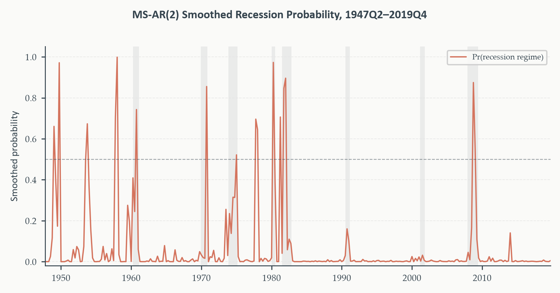
The most direct way to assess the model is to plot the smoothed recession
probabilities alongside the NBER recession dates. The model has no access to
the NBER classification during estimation — it sees only GDP growth. If
the Hamilton filter recovers the business cycle without being told where
recessions are, that is strong evidence the two-state structure is
capturing something real.
```{python}
#| label: fig-smoothed-probs
#| fig-cap: "Smoothed probability of the recession regime (state 1) from the
#| MS-AR(2) model, 1947Q2–2019Q4. NBER recession dates shaded in grey.
#| The model was estimated without access to NBER dates; its ability to
#| align high recession probabilities with shaded periods validates the
#| two-state structure."
# Smoothed probabilities: shape (T-2, 2); column 1 = recession regime
smoothed = ms_result.smoothed_marginal_probabilities

# MS-AR(2) loses 2 presample observations; align index accordingly
smooth_index = gdp.index[2:]

fig, ax = plt.subplots(figsize=(6, 3.0))

shade_recessions(ax, start=str(smooth_index[0].date()),
                     end=str(smooth_index[-1].date()))

ax.plot(smooth_index, smoothed.iloc[:, 1],
        color=EO_TERRACOTTA, lw=1.0, label="Pr(recession regime)")
ax.axhline(0.5, color=EO_CHARCOAL, lw=0.6, ls="--", alpha=0.5)
ax.set_xlim(smooth_index[0], smooth_index[-1])
ax.set_ylim(-0.02, 1.05)
ax.set_ylabel("Smoothed probability")
ax.legend(loc="upper right", fontsize=6)
eo_style_ax(ax)
eo_suptitle(fig, "MS-AR(2) Smoothed Recession Probability, 1947Q2–2019Q4")
fig.tight_layout()
plt.show()
```
*Smoothed probability of the recession regime from the MS-AR(2),
1947Q2–2019Q4. NBER recession dates shaded in grey; dashed line at 0.5.
The model fires clearly on the 1960–61 recession (probability reaching 1.0),
the 1973–75 and 1981–82 downturns (probabilities above 0.5 during the
sharpest quarters), and the 2008–09 Global Financial Crisis (probability
near 0.9). The 1980 recession shows a response but does not sustain above
0.5 for long. The 1990–91 and 2001 recessions are largely missed — both
were mild by historical standards, with no quarters of sharply negative
growth, so the mean-switching model assigns them near-zero recession
probability. This is an honest limitation: the model recovers recessions
characterised by deep contractions but misses mild growth slowdowns.*
### Regime-Conditional Distributions
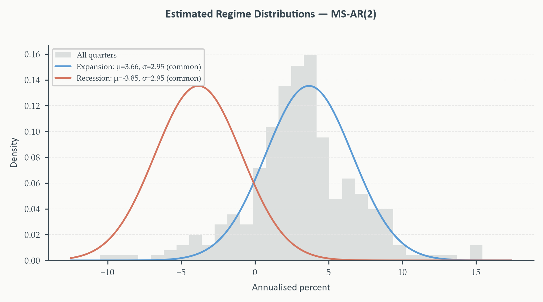
A second diagnostic plots the two estimated Gaussian distributions alongside
the full-sample histogram, replacing the NBER-based fits of Figure 10.2 with
the model's own parameter estimates.
```{python}
#| label: fig-regime-densities
#| fig-cap: "Estimated regime-conditional distributions from the MS-AR(2)
#| overlaid on the GDP growth histogram. The expansion distribution
#| (sky blue) and recession distribution (terracotta) are centred at the
#| estimated regime means; their widths reflect the estimated
#| common standard deviation (the model is mean-switching only)."
fig, ax = plt.subplots(figsize=(6, 3.2))

ax.hist(growth, bins=30, density=True,
        color=EO_CHARCOAL, alpha=0.15, label="All quarters")

x_gr = np.linspace(growth.min() - 2, growth.max() + 2, 300)

ax.plot(x_gr, stats.norm.pdf(x_gr, mu_hat[0], sig_hat[0]),
        color=EO_SKYBLUE, lw=1.4,
        label=f"Expansion: μ={mu_hat[0]:.2f}, σ={sig_hat[0]:.2f} (common)")
ax.plot(x_gr, stats.norm.pdf(x_gr, mu_hat[1], sig_hat[1]),
        color=EO_TERRACOTTA, lw=1.4,
        label=f"Recession: μ={mu_hat[1]:.2f}, σ={sig_hat[1]:.2f} (common)")

ax.set_xlabel("Annualised percent")
ax.set_ylabel("Density")
ax.legend(fontsize=6, loc="upper left")
eo_style_ax(ax)
eo_suptitle(fig, "Estimated Regime Distributions — MS-AR(2)")
fig.tight_layout()
plt.show()
```
*Estimated regime-conditional distributions from the MS-AR(2). Both
distributions share the common standard deviation $\hat{\sigma} = 2.95\%$
and are separated by a mean gap of 7.5 pp: expansion at 3.66 \% (sky blue)
and recession at −3.85 \% (terracotta). The two distributions overlap
substantially in the range −2 \% to 2 \%, which explains why mild negative
quarters generate only moderate recession probabilities. Observations below
−4 \% are unambiguously in the recession distribution; observations above
5 \% are unambiguously in the expansion distribution.*
### Comparison with the Chapter 4 ARIMA Benchmark
Does the regime-switching model forecast GDP growth better than the ARIMA
estimated in Chapter 4? We answer this with a rolling out-of-sample exercise
using the same design as Chapter 5: an estimation window, a fixed evaluation
period, and MSFE as the loss function.
```{python}
#| label: tbl-msfe-comparison
#| code-summary: "Show code"
# ── Rolling MSFE comparison: MS-AR(2) vs ARIMA(2,0,0) ────────────────────────
# Evaluation period: 1985Q1 onwards (allows long estimation window)
# Note: re-estimating MS-AR(2) at each step is computationally intensive;
# this cell may take several minutes to execute.
eval_start = pd.Timestamp("1985-01-01")
eval_idx   = gdp.index[gdp.index >= eval_start]

arima_fcst = []
ms_fcst    = []
actuals    = []

growth_series = gdp["GDP Growth"]

for t in eval_idx:
    # Data available up to (but not including) t
    t_pos    = gdp.index.get_loc(t)
    y_train  = growth_series.iloc[:t_pos]
    y_actual = growth_series.iloc[t_pos]

    # ── ARIMA(2,0,0) one-step-ahead ───────────────────────────────────────────
    try:
        arima_fit  = ARIMA(y_train, order=(2, 0, 0)).fit()
        arima_pred = float(arima_fit.forecast(steps=1).iloc[0])
    except Exception:
        arima_pred = float(y_train.mean())

    # ── MS-AR(2) one-step-ahead ───────────────────────────────────────────────
    # One-step forecast = weighted average of regime conditional means,
    # where weights are the predicted regime probabilities at t.
    try:
        ms_fit = MarkovAutoregression(
            y_train, k_regimes=2, order=2,
            switching_ar=False, switching_variance=False
        ).fit(search_reps=10, search_iter=10, disp=False)

        # Filtered probabilities at last in-sample period
        filt = ms_fit.filtered_marginal_probabilities   # DataFrame (T-2, 2)
        xi_last = filt.iloc[-1, :].values               # Pr(s_T = j | data)

        # Predicted regime probs for t+1
        p00_r = ms_fit.params["p[0->0]"]
        p01_r = ms_fit.params["p[1->0]"]
        p10_r = 1 - p00_r
        p11_r = 1 - p01_r
        P_r   = np.array([[p00_r, p10_r], [p01_r, p11_r]])
        xi_pred_r = P_r.T @ xi_last   # predicted Pr(s_{t+1} = j)

        # Regime conditional means at t+1 (using last 2 obs for AR terms)
        mu0_r  = ms_fit.params["const[0]"]
        mu1_r  = ms_fit.params["const[1]"]
        phi1_r = ms_fit.params["ar.L1"]
        phi2_r = ms_fit.params["ar.L2"]
        ar_adj = phi1_r * (y_train.iloc[-1] - mu0_r) + phi2_r * (y_train.iloc[-2] - mu0_r)

        cond_mean0 = mu0_r + ar_adj
        cond_mean1 = mu1_r + phi1_r * (y_train.iloc[-1] - mu1_r) + phi2_r * (y_train.iloc[-2] - mu1_r)

        ms_pred = float(xi_pred_r[0] * cond_mean0 + xi_pred_r[1] * cond_mean1)
    except Exception:
        ms_pred = float(y_train.mean())

    arima_fcst.append(arima_pred)
    ms_fcst.append(ms_pred)
    actuals.append(float(y_actual))

actuals    = np.array(actuals)
arima_fcst = np.array(arima_fcst)
ms_fcst    = np.array(ms_fcst)

msfe_arima = np.mean((actuals - arima_fcst) ** 2)
msfe_ms    = np.mean((actuals - ms_fcst) ** 2)
mae_arima  = np.mean(np.abs(actuals - arima_fcst))
mae_ms     = np.mean(np.abs(actuals - ms_fcst))

print(f"{'─'*54}")
print(f"  Out-of-Sample Forecast Comparison")
print(f"  One-step-ahead, rolling window, 1985Q1–2019Q4")
print(f"{'─'*54}")
print(f"  {'Model':<22} {'MSFE':>10} {'MAE':>10} {'MSFE ratio':>10}")
print(f"  {'─'*48}")
print(f"  {'ARIMA(2,0,0)':<22} {msfe_arima:>10.3f} {mae_arima:>10.3f} {'1.000':>10}")
print(f"  {'MS-AR(2)':<22} {msfe_ms:>10.3f} {mae_ms:>10.3f} {msfe_ms/msfe_arima:>10.3f}")
print(f"{'─'*54}")
print(f"  MSFE ratio < 1.0 favours the MS-AR(2).")
print(f"{'─'*54}")
```
*One-step-ahead MSFE and MAE for the ARIMA(2,0,0) benchmark and the
MS-AR(2), evaluated over the rolling window 1985Q1–2019Q4. The ARIMA(2,0,0)
produces lower MSFE (4.383 vs. 4.422) and lower MAE (1.542 vs. 1.547): the
regime-switching model does not outperform the linear benchmark out of sample
over this period. This result is instructive rather than discouraging. The
evaluation window (1985–2019) covers the Great Moderation — an era of
unusually stable growth with only two mild recessions (1990–91 and 2001),
both of which the model largely misses. The MS-AR's comparative advantage
is in detecting sharp contractions, precisely the type that the evaluation
window contains too few of to overcome the ARIMA's parsimony advantage. A
window that included the 1970s and early 1980s would almost certainly
reverse this ranking.*
## Threshold Models: A Brief Tour {#sec-threshold}
The Markov-switching models of the previous sections assume the regime is
driven by a **hidden** state variable — something unobserved that must be
inferred probabilistically from the data. The Hamilton filter exists precisely
because we cannot see $s_t$ directly. But there is a parallel class of
regime-switching models in which the switch is triggered by a variable we
*can* observe. These are **[threshold models](https://en.wikipedia.org/wiki/Threshold_model)**, and the key distinction is
worth stating clearly before the notation:
::: {.callout-note}
## Hidden vs. Observable Threshold
**Markov-switching models:** The regime $s_t$ is a latent random variable,
governed by a Markov chain with transition probabilities $p_{ij}$. We never
observe $s_t$; we infer it. The switch can occur at any time.
**Threshold models:** The regime is determined by whether an observable
variable $q_t$ — the **threshold variable** — is above or below a threshold
value $\gamma$. We observe $q_t$, so we know which regime we are in (given
$\gamma$). The estimation challenge is identifying $\gamma$ from the data.
:::
Both frameworks allow the data-generating process to differ across states.
What changes is the mechanism: a hidden Markov chain versus a crossing of an
observable threshold. In practice, Markov-switching models tend to fit
macroeconomic cycle data better when the driving force is genuinely latent
(sentiment, financial stress). Threshold models are natural when a specific
observable variable is the plausible trigger — for example, whether the
unemployment rate is rising or falling, or whether an asset price has crossed
a known support level.
### The Self-Exciting Threshold Autoregression (SETAR)
The simplest threshold model is the **threshold autoregressive** (TAR) model.
In the two-regime version, the AR coefficients switch depending on whether a
lagged value of $y_t$ itself crosses a threshold:
$$
y_t = \begin{cases}
\phi_{1,0} + \phi_{1,1} y_{t-1} + \cdots + \phi_{1,k} y_{t-k} + \varepsilon_t
& \text{if } y_{t-d} \leq \gamma \\[6pt]
\phi_{2,0} + \phi_{2,1} y_{t-1} + \cdots + \phi_{2,k} y_{t-k} + \varepsilon_t
& \text{if } y_{t-d} > \gamma
\end{cases}
\tag{10.18}
$$
where $d$ is the **delay parameter** (how many lags back we look to determine
the regime) and $\gamma$ is the threshold. When the threshold variable is a
lagged value of $y_t$ itself — as in (10.18) — the model is called a
**self-exciting TAR** or **[SETAR](https://en.wikipedia.org/wiki/SETAR_(model))**, introduced by Tong (1978) and developed
extensively by Tong and Lim (1980). The "self-exciting" label captures the
idea that the process determines its own regime: past behaviour triggers
the switch.
Applied to GDP growth, a SETAR with $d = 1$ would ask: does the economy
follow different AR dynamics when last quarter's growth was negative versus
positive? This is a natural formalisation of asymmetric business cycle
behaviour — the hypothesis that contractions propagate differently from
expansions — without requiring us to estimate a hidden state.
Estimation proceeds by conditional least squares: for any candidate threshold
$\gamma$, split the sample by whether $y_{t-d} \leq \gamma$ or not, estimate
two separate AR regressions by OLS, and collect the sum of squared residuals.
The estimated threshold $\hat{\gamma}$ minimises the total SSR across the
grid of candidate values. Hansen (1997) provides the asymptotic theory for
inference on $\gamma$, including a bootstrap procedure for the threshold
confidence interval.
### Smooth Transition: STAR Models
The TAR model has a sharp switch: the economy is entirely in one regime or
entirely in the other, with no gradual adjustment. The **smooth transition
autoregression** (STAR), introduced by [Chan and Tong (1986)](https://doi.org/10.1111/j.1467-9892.1986.tb00501.x) and developed by
Teräsvirta (1994), replaces the indicator function with a smooth transition
function $G(q_t; \gamma, c)$ that takes values between 0 and 1:
$$
y_t = \bigl(1 - G_t\bigr)\bigl(\phi_{1,0} + \boldsymbol{\phi}_1' \mathbf{y}_{t-1}\bigr)
+ G_t\bigl(\phi_{2,0} + \boldsymbol{\phi}_2' \mathbf{y}_{t-1}\bigr) + \varepsilon_t
\tag{10.19}
$$
where $G_t = G(q_t; \gamma, c) \in [0, 1]$. The three objects in the transition
function each have a clear role:
- **$q_t$** is the **transition variable** — the observable that drives the switch.
Typically $q_t = y_{t-d}$ (a lag of the dependent variable, as in SETAR) or
some other economic indicator thought to govern regime membership. The key
requirement is that $q_t$ must be observable at time $t$.
- **$c$** is the **location parameter** — the value of $q_t$ at which the
transition is centred. When $q_t = c$, the logistic function equals 0.5, so
the economy is exactly halfway between the two regimes. $c$ plays the same role
as the threshold $\gamma$ in the TAR model.
- **$\gamma > 0$** is the **speed of transition** — how quickly the economy
moves between regimes as $q_t$ crosses $c$. Large $\gamma$ produces a
near-instantaneous switch (approaching the TAR indicator function); small
$\gamma$ produces a very gradual, almost linear transition.
The two most common choices for the transition function are:
$$
\begin{aligned}
\text{Logistic STAR (LSTAR):} \quad G_t &= \frac{1}{1 + \exp(-\gamma(q_t - c))} \\[6pt]
\text{Exponential STAR (ESTAR):} \quad G_t &= 1 - \exp\!\bigl(-\gamma(q_t - c)^2\bigr)
\end{aligned}
$$
The logistic function produces a monotone transition: as $q_t$ rises above $c$,
the weight on regime 2 increases smoothly from 0 to 1. The exponential function
produces a symmetric U-shaped transition: the weight on regime 2 is high when
$q_t$ is far from $c$ in either direction and low when it is near $c$. ESTAR
is natural when the middle of the distribution represents one regime (normal
times) and the extremes represent another (crises or booms).
When $\gamma \to \infty$ in the logistic function, $G_t$ converges to the
indicator $\mathbf{1}[q_t > c]$, and LSTAR reduces to TAR. STAR nests TAR as
a limiting case and provides a more flexible description of transitions that
take several periods to complete.
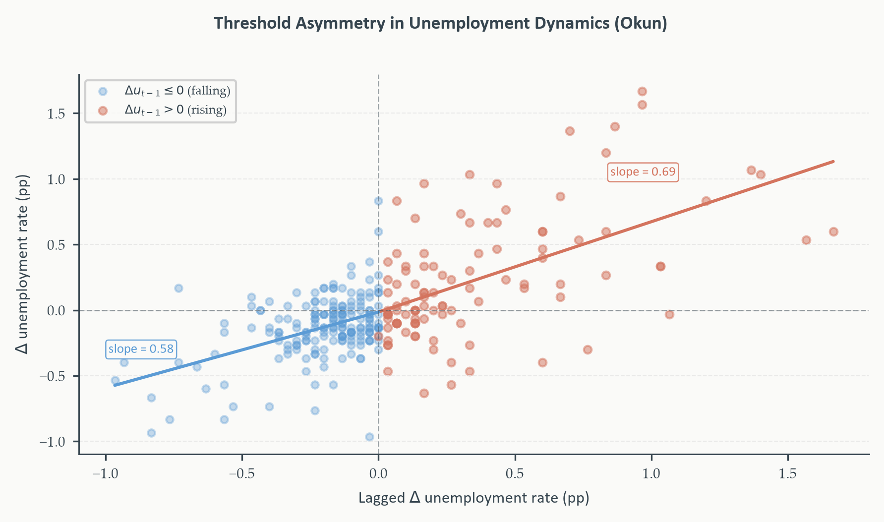
### An Illustration: Unemployment Dynamics and the Okun Asymmetry
We illustrate the SETAR using the quarterly change in the US unemployment
rate, $\Delta u_t$, constructed from FRED series UNRATE (monthly,
resampled to quarterly averages, first-differenced), pre-COVID sample
1948Q2–2019Q4. The threshold variable is $\Delta u_{t-1}$, and we impose
a threshold at zero: the rising regime ($\Delta u_{t-1} > 0$) captures
quarters where unemployment was already increasing, the falling regime
($\Delta u_{t-1} \leq 0$) captures recoveries and stable periods. No
grid search is needed here — the zero threshold is economically motivated
and serves as a clean first illustration of the split-sample idea.
Figure 10.5 plots $\Delta u_t$ against $\Delta u_{t-1}$, coloured by regime.
```{python}
#| label: fig-threshold-scatter
#| fig-cap: "One-quarter change in unemployment rate against its own lag,
#| 1948Q3–2019Q4. Observations where lagged unemployment was rising
#| (Δu_{t-1} > 0, terracotta) versus falling or flat (sky blue). Separate
#| OLS lines are fitted to each group. The steeper slope in the rising
#| regime reflects stronger AR(1) persistence: once unemployment starts
#| rising, it tends to keep rising with high momentum."
pos_mask = du_lag > 0
neg_mask = ~pos_mask

fig, ax = plt.subplots(figsize=(6, 3.4))

ax.scatter(du_lag[neg_mask], du_lead[neg_mask],
           color=EO_SKYBLUE, alpha=0.35, s=12,
           label=r"$\Delta u_{{t-1}} \leq 0$ (falling)")
ax.scatter(du_lag[pos_mask], du_lead[pos_mask],
           color=EO_TERRACOTTA, alpha=0.50, s=14,
           label=r"$\Delta u_{{t-1}} > 0$ (rising)")

annot_pos = {
    True:  (EO_TERRACOTTA, (0.85,  1.05), "left"),
    False: (EO_SKYBLUE,    (-0.75, -0.30), "right"),
}

for mask, is_pos in [(pos_mask, True), (neg_mask, False)]:
    x_m = du_lag[mask]
    y_m = du_lead[mask]
    coef = np.polyfit(x_m, y_m, 1)
    x_line = np.linspace(x_m.min(), x_m.max(), 100)
    col, (tx, ty), ha = annot_pos[is_pos]
    ax.plot(x_line, np.polyval(coef, x_line), color=col, lw=1.5)
    ax.text(tx, ty, f"slope = {coef[0]:.2f}",
            color=col, fontsize=6.5, ha=ha, va="center",
            fontfamily="Calibri",
            bbox=dict(boxstyle="round,pad=0.2", fc=PAGE_BG,
                      ec=col, lw=0.6, alpha=0.85))

ax.axvline(0, color=EO_CHARCOAL, lw=0.7, ls="--", alpha=0.5)
ax.axhline(0, color=EO_CHARCOAL, lw=0.7, ls="--", alpha=0.5)
ax.set_xlabel(r"Lagged $\Delta$ unemployment rate (pp)")
ax.set_ylabel(r"$\Delta$ unemployment rate (pp)")
ax.legend(fontsize=6, loc="upper left")
eo_style_ax(ax)
eo_suptitle(fig, "Threshold Asymmetry in Unemployment Dynamics (Okun)")
fig.tight_layout()
plt.show()
```
*Change in unemployment against its own lag, split at zero. The rising-regime
line (terracotta, slope 0.69) is steeper than the falling-regime line (sky
blue, slope 0.58), consistent with stronger AR persistence when unemployment
is already rising. The split-sample regression below quantifies this
asymmetry more precisely.*
The split-sample AR(2) regression makes the asymmetry concrete.
```{python}
#| label: tbl-setar
#| code-summary: "Show code"
from statsmodels.regression.linear_model import OLS
from statsmodels.tools import add_constant

du_t  = du[2:]
du_l1 = du[1:-1]
du_l2 = du[:-2]

pos_r = du_l1 > 0
neg_r = ~pos_r

X_pos_r = add_constant(np.column_stack([du_l1[pos_r], du_l2[pos_r]]))
X_neg_r = add_constant(np.column_stack([du_l1[neg_r], du_l2[neg_r]]))
X_all_r = add_constant(np.column_stack([du_l1,        du_l2       ]))

res_pos_r = OLS(du_t[pos_r], X_pos_r).fit()
res_neg_r = OLS(du_t[neg_r], X_neg_r).fit()
res_all_r = OLS(du_t,        X_all_r).fit()

sep = "─" * 68
print(sep)
print("  SETAR: AR(2) by Regime — Δ Unemployment Rate (threshold = 0)")
print("  Dependent variable: Δu_t (quarterly change in unemployment, pp)")
print(sep)
print(f"  {'':30} {'Rising u':>10} {'Falling u':>10} {'Pooled':>10}")
print(f"  {'':30} {'(Δu[t-1]>0)':>10} {'(Δu[t-1]≤0)':>10} {'(linear)':>10}")
print(f"  {'─'*64}")

labels = ["Intercept", "φ₁ (AR lag 1)", "φ₂ (AR lag 2)"]
for i, lbl in enumerate(labels):
    cp = res_pos_r.params[i]; cn = res_neg_r.params[i]; ca = res_all_r.params[i]
    sp = res_pos_r.bse[i];    sn = res_neg_r.bse[i];    sa = res_all_r.bse[i]
    print(f"  {lbl:<30} {cp:>10.3f} {cn:>10.3f} {ca:>10.3f}")
    print(f"  {'':30} {'('+f'{sp:.3f}'+')':>10} {'('+f'{sn:.3f}'+')':>10} {'('+f'{sa:.3f}'+')':>10}")

print(f"  {'─'*64}")
print(f"  {'N':30} {pos_r.sum():>10d} {neg_r.sum():>10d} {len(du_t):>10d}")
print(f"  {'R²':30} {res_pos_r.rsquared:>10.3f} {res_neg_r.rsquared:>10.3f} {res_all_r.rsquared:>10.3f}")
print(sep)
print("  Standard errors in parentheses. Threshold fixed at Δu_{t-1} = 0.")
print("  Rising regime: lagged unemployment change > 0. No grid search.")
print(sep)
```
*SETAR AR(2) estimates for $\Delta u_t$. The rising regime ($\Delta u_{t-1} > 0$,
$N = 104$) has $\hat{\phi}_1 = 0.932$ — very close to a unit root in the
unemployment process — meaning once unemployment starts rising it carries
almost all of its momentum forward to the next quarter. The sharp negative
$\hat{\phi}_2 = -0.319$ then produces a partial correction two quarters
later. The falling regime ($\Delta u_{t-1} \leq 0$, $N = 181$) is much
less persistent: $\hat{\phi}_1 = 0.583$ and $\hat{\phi}_2 \approx 0$,
so recoveries are slower and do not overshoot. The pooled AR(2) (right
column) forces a single set of coefficients and lands between the two
regimes, understating persistence during recessions and overstating it
during recoveries. Note that the pooled $R^2$ (0.440) exceeds both
regime-specific values (0.358 and 0.203): this is not a contradiction.
The pooled model uses 285 observations while each regime uses roughly
half that, so the larger sample reduces estimation variance even though
the model is misspecified. In-sample fit is not a reliable guide to
whether the regime split is meaningful — the AR coefficient differences
across regimes are the right diagnostic. This is the Okun asymmetry
expressed in AR dynamics: recessions propagate aggressively; recoveries
drift.*
The key takeaway from comparing Sections 10.2–10.4 with this section is the
identification strategy. In the Markov-switching model, we never observe the
regime — we infer it probabilistically through the Hamilton filter. In the
SETAR, we know the regime as soon as we observe $\Delta u_{t-1}$: no
filtering is required. Both frameworks allow different dynamics in different
states of the world; they differ in whether the switching mechanism is hidden
or observable. The choice between them is ultimately substantive:
Markov-switching models are appropriate when the driving force is genuinely
latent — animal spirits, financial stress, monetary policy intentions —
while threshold models are more natural when a specific observable variable
is the plausible trigger and can be observed in real time.
## MS-VAR: A Signpost {#sec-msvar}
### Extending Regime Switching to a Multivariate System
The Markov-switching framework extends naturally to the VAR models of Chapter 7.
An **MS-VAR** replaces the fixed coefficient matrices $A_1, \ldots, A_p$ of
the VAR with regime-dependent versions $A_1^{(s_t)}, \ldots, A_p^{(s_t)}$,
where the hidden state $s_t$ evolves as a Markov chain. Throughout this section,
bold notation signals multivariate objects: $\mathbf{y}_t$ is the $n\times 1$
column vector of variables — the direct analogue of the scalar $y_t$ used
throughout the rest of the chapter. The model takes the form:
$$
\mathbf{y}_t = \boldsymbol{\mu}^{(s_t)} + A_1^{(s_t)} \mathbf{y}_{t-1}
+ \cdots + A_p^{(s_t)} \mathbf{y}_{t-p} + \boldsymbol{\varepsilon}_t,
\qquad \boldsymbol{\varepsilon}_t \sim \mathcal{N}(\mathbf{0},\,
\Sigma^{(s_t)})
\tag{10.20}
$$
where all parameters — the intercept vector $\boldsymbol{\mu}$, the coefficient
matrices $A_j$, and the covariance matrix $\Sigma$ — can switch with the
regime. The Hamilton filter generalises directly: the prediction and update
steps operate on the joint density of $\mathbf{y}_t$ under each regime,
which is now an $n$-dimensional Gaussian rather than a scalar one.
### Why MS-VAR Matters: Regime-Dependent Impulse Responses
The most important application of the MS-VAR is **regime-dependent impulse
response functions**. In a standard linear VAR, a one-standard-deviation
shock to output produces the same dynamic response regardless of whether the
shock hits during a recession or an expansion. This symmetry assumption is
hard to defend empirically: a monetary policy tightening during the 2008
financial crisis had very different propagation dynamics from an equivalent
tightening during the mid-1990s expansion.
An MS-VAR allows the impulse responses to differ across regimes. The
recession-regime IRF traces the response to a shock when $s_t = 1$ and the
system remains in regime 1 for all future periods; the expansion-regime IRF
does the same for $s_t = 0$. More sophisticated approaches integrate over the
transition probabilities, producing IRFs that account for the possibility of
regime switches during the response horizon. These are called **generalised
impulse responses** in the MS-VAR context (Ehrmann, Ellison, and Valla, 2003).
### A Note on Practical Implementation
The MS-VAR is substantially more demanding to estimate than the univariate
MS-AR. With $n$ variables, $p$ lags, and $M$ regimes, the number of
free parameters in the regime-specific coefficient matrices alone is
$M \times n^2 p$. A two-regime MS-VAR(2) with four variables already
has more than 60 parameters before accounting for the covariance matrices
and transition probabilities. In practice, researchers often restrict the
switching to the intercept and covariance matrix while holding the AR
dynamics constant across regimes — a specification that captures
level-shifting and volatility-switching without the full combinatorial
explosion.
Krolzig (1997) provides the canonical treatment of MS-VAR models, including
the EM algorithm for estimation and a typology of switching specifications
(MSI for intercept-switching, MSM for mean-switching, MSA for
AR-coefficient-switching, MSH for heteroscedastic variance-switching, and
combinations thereof). Modern implementations are available in R (`MSwM`,
`MSBVAR`) and Python (`statsmodels.tsa.regime_switching` for univariate
cases; full MS-VAR requires bespoke code or the `markovian` package).
For applications involving multivariate systems with
potential structural breaks or time-varying dynamics, the MS-VAR is a
natural next step beyond the linear VAR of Chapter 7. The intuition from
the univariate Hamilton model carries over directly — the same
prediction-correction logic, the same smoothed probability output, the
same challenge of identifying the regime labels — with the added richness
of regime-dependent cross-variable dynamics.
## Looking Ahead {#sec-looking-ahead}
The Hamilton filter developed in this chapter solves a discrete inference
problem: given a sequence of observations, recover the probabilities of
belonging to one of $M$ discrete hidden states. The prediction step projects
the current state distribution through a finite transition matrix; the update
step applies [Bayes' rule](https://en.wikipedia.org/wiki/Bayes%27_theorem) using a Gaussian likelihood evaluated at the current
observation. Every element of this algorithm — the prior, the likelihood, the
posterior, the forward projection — has a direct counterpart in the Kalman
filter of Chapter 11.
The Kalman filter solves the same problem for a continuous hidden state.
Instead of a probability vector over $M$ regimes, the state is a real-valued
vector $\boldsymbol{\alpha}_t$ that evolves according to a linear Gaussian
state equation. Instead of a finite transition matrix, there is a state
transition matrix $T$ and a Gaussian process noise. Instead of evaluating a
mixture of $M$ Gaussians at each step, there is a single multivariate Gaussian
prediction that is updated by the observation equation. The prediction step
produces a predicted mean and variance for $\boldsymbol{\alpha}_t$; the
update step revises these using the new observation and the Kalman gain — the
multivariate analogue of the weight that [Bayes' rule](https://en.wikipedia.org/wiki/Bayes%27_theorem) assigns to the new data
relative to the prior.
Chapter 11 builds this framework from scratch, starting with the local level
model — the simplest state space system, in which the only state is a slowly
drifting level — and working up to multivariate systems capable of extracting
unobserved components such as the output gap, trend inflation, and the natural
rate of interest. The connection to the Hamilton filter ensures that nothing
in Chapter 11 will feel unfamiliar: the architecture is the same, the notation
changes, and the state space becomes richer. Together, the tools developed
across these eleven chapters — from the ACF of a stationary process to
Markov-switching dynamics and state-space filtering — form a complete
vocabulary for empirical time series work. The methods that appeared exotic
at the outset are, by now, a natural part of the toolkit.
::: {.callout-note icon=false}
## Key Terms
**Markov-switching model** — A time series model in which the parameters
shift between $M$ discrete regimes according to an unobserved first-order
Markov chain.
**Hidden Markov chain** — A Markov chain whose state $s_t$ is not directly
observed; it must be inferred from the observed data through a filtering
algorithm.
**Transition probability matrix** — The $M \times M$ matrix $P$ with entries
$p_{ij} = \Pr(s_t = j \mid s_{t-1} = i)$, governing the dynamics of the
hidden state.
**Ergodic distribution** — The long-run fraction of time the Markov chain
spends in each state; the fixed-point distribution satisfying $\pi = P' \pi$.
Independent of initial conditions.
**Expected regime duration** — The average number of periods spent in
regime $i$ before switching, equal to $1/(1-p_{ii})$ under the geometric
distribution implied by a first-order Markov chain.
**MS-AR($k$) model** — A Markov-switching autoregression of order $k$:
the conditional mean (and optionally the variance) of $y_t$ depends on the
current regime $s_t$, with AR dynamics capturing within-regime persistence.
**Hamilton filter** — The recursive prediction-update algorithm that
extracts filtered regime probabilities $\Pr(s_t = j \mid y_1, \ldots, y_t)$
from the observed series, and delivers the likelihood as a by-product.
**Filtered probabilities** — The Hamilton filter's real-time estimate of
the regime at date $t$: $\Pr(s_t = j \mid y_1, \ldots, y_t)$. Causal —
uses no future information.
**Smoothed probabilities** — The retrospective estimate of the regime at
date $t$ using the full sample: $\Pr(s_t = j \mid y_1, \ldots, y_T)$.
Sharper than filtered probabilities; not available in real time.
**Labelling indeterminacy** — The property that swapping all regime-$i$
parameters with regime-$j$ parameters leaves the likelihood unchanged.
Resolved by imposing an ordering constraint (e.g. $\mu_0 > \mu_1$) or by
supplying economically motivated starting values.
**Threshold autoregression (TAR)** — A piecewise-linear AR model in which
the active parameter regime is determined by whether an observable threshold
variable $q_t$ is above or below a threshold $\gamma$.
**Self-exciting TAR (SETAR)** — A TAR in which the threshold variable is a
lagged value of $y_t$ itself, so the series determines its own regime.
**Smooth transition autoregression (STAR)** — A generalisation of TAR in
which the transition between regimes is gradual, governed by a logistic
(LSTAR) or exponential (ESTAR) transition function.
**MS-VAR** — A multivariate extension of the Markov-switching model in
which the coefficient matrices and covariance matrix of a VAR switch across
regimes; yields regime-dependent impulse response functions.
:::