---
title: "Volatility Models — ARCH, GARCH, and Extensions"
author: ""
abstract: |
Every model in Chapters 3 through 8 targeted the conditional mean of a time
series: we asked what the best point forecast of tomorrow's value is, given
what we know today. This chapter asks a different question — and the answer
turns out to be economically more interesting than it first appears. For
financial asset returns, the conditional mean is nearly unforecastable.
Markets aggregate information so efficiently that there is almost no
predictable component in the average daily return on the S&P 500. But the
*variance* of that return — how uncertain the next day's outcome is — is
highly forecastable. Calm markets tend to remain calm; turbulent ones tend
to remain turbulent. This phenomenon, known as volatility clustering, is the
central empirical fact that motivates everything in this chapter. We begin
with the Efficient Market Hypothesis and its implication that returns should
be unpredictable, then show immediately that squared returns are not: the
second moment has memory even when the first does not. That observation leads
to Engle's ARCH model and its elegant extension, the GARCH(1,1), which
captures volatility dynamics with just three parameters. We then examine
asymmetric volatility — the leverage effect that makes bad news more
destabilising than equally sized good news — through the GJR-GARCH and
EGARCH models. The chapter closes with two practical applications: Dynamic
Conditional Correlation for portfolio risk and GARCH-based Value at Risk.
Throughout, the running example is daily S&P 500 log returns from 1980
through 2019, a sample that contains Black Monday, the Asian and Russian
crises, the dot-com bust, and the Global Financial Crisis — exactly the
volatility episodes that GARCH models were built to handle.
jupyter: python3
format:
html:
toc: true
toc-depth: 3
toc-title: "In this chapter"
number-sections: true
code-fold: true
code-summary: "Show code"
code-tools: true
theme: cosmo
css: styles.css
highlight-style: github
fig-align: center
fig-cap-location: bottom
fig-responsive: true
html-math-method: mathjax
embed-resources: false
execute:
echo: true
warning: false
message: false
cache: false
---
```{python}
#| label: install
#| include: false
import subprocess, sys
subprocess.run([sys.executable, "-m", "pip", "install", "--quiet",
"--break-system-packages", "yfinance", "arch"],
check=True)
```
```{python}
#| label: setup
#| include: false
import numpy as np
import pandas as pd
import matplotlib.pyplot as plt
import matplotlib as mpl
import matplotlib.ticker as mticker
import yfinance as yf
from arch import arch_model
from statsmodels.stats.diagnostic import acorr_ljungbox
from statsmodels.tsa.stattools import acf
from scipy import stats
from datetime import datetime
import warnings
warnings.filterwarnings("ignore")
# ── EO Brand Palette ───────────────────────────────────────────────────────────
EO_CHARCOAL = "#36454F"
EO_COPPER = "#B87333"
EO_SAGE = "#87A96B"
EO_SKYBLUE = "#5B9BD5"
EO_TERRACOTTA = "#D4745E"
EO_LAVENDER = "#8E7AB5"
EO_COLORS = [EO_COPPER, EO_SKYBLUE, EO_SAGE,
EO_TERRACOTTA, EO_LAVENDER, EO_CHARCOAL]
PAGE_BG = "#FAFAF8"
# ── Global rcParams ────────────────────────────────────────────────────────────
mpl.rcParams.update({
"figure.figsize": (6, 3),
"figure.dpi": 150,
"figure.facecolor": PAGE_BG,
"figure.edgecolor": PAGE_BG,
"axes.facecolor": PAGE_BG,
"axes.edgecolor": EO_CHARCOAL,
"axes.linewidth": 0.7,
"axes.grid": True,
"axes.grid.axis": "y",
"axes.spines.top": False,
"axes.spines.right": False,
"axes.titlesize": 9,
"axes.titleweight": "bold",
"axes.titlecolor": EO_CHARCOAL,
"axes.titlelocation": "left",
"axes.labelsize": 8,
"axes.labelcolor": EO_CHARCOAL,
"axes.labelweight": "normal",
"axes.prop_cycle": mpl.cycler(color=EO_COLORS),
"grid.color": "#E5E5E5",
"grid.linewidth": 0.5,
"grid.linestyle": "--",
"grid.alpha": 0.8,
"xtick.color": EO_CHARCOAL,
"ytick.color": EO_CHARCOAL,
"xtick.labelsize": 7,
"ytick.labelsize": 7,
"xtick.direction": "out",
"ytick.direction": "out",
"xtick.major.size": 3,
"ytick.major.size": 3,
"lines.linewidth": 1.2,
"lines.solid_capstyle": "round",
"legend.frameon": True,
"legend.framealpha": 0.9,
"legend.edgecolor": "#CCCCCC",
"legend.facecolor": PAGE_BG,
"legend.fontsize": 6,
"legend.title_fontsize": 6,
"font.family": "serif",
"font.serif": ["Palatino Linotype", "Palatino", "Georgia",
"DejaVu Serif"],
"font.sans-serif": ["Calibri", "Arial", "DejaVu Sans"],
"font.size": 8,
"text.color": EO_CHARCOAL,
"savefig.dpi": 300,
"savefig.bbox": "tight",
"savefig.facecolor": PAGE_BG,
})
def eo_suptitle(fig, title, **kwargs):
defaults = dict(fontsize=9, fontweight="bold",
color=EO_CHARCOAL, fontfamily="Calibri", y=1.01)
defaults.update(kwargs)
fig.suptitle(title, **defaults)
def eo_style_ax(ax):
for obj in [ax.title, ax.xaxis.label, ax.yaxis.label]:
obj.set_fontfamily("Calibri")
# NBER recession dates
RECESSIONS = [
("1980-01-01", "1980-07-01"),
("1981-07-01", "1982-11-01"),
("1990-07-01", "1991-03-01"),
("2001-03-01", "2001-11-01"),
("2007-12-01", "2009-06-01"),
]
def shade_recessions(ax, start=None, end=None):
for rec_start, rec_end in RECESSIONS:
s, e = pd.Timestamp(rec_start), pd.Timestamp(rec_end)
if start is not None and e < pd.Timestamp(start):
continue
if end is not None and s > pd.Timestamp(end):
continue
ax.axvspan(s, e, color=EO_CHARCOAL, alpha=0.08, lw=0)
```
```{python}
#| label: data-download
#| include: false
#| cache: true
from pathlib import Path
DATA_PATH = Path("../../data/raw")
# ── S&P 500 daily prices from local CSV ───────────────────────────────────────
sp500_raw = pd.read_csv(DATA_PATH / "SP500.csv", index_col="date", parse_dates=True).loc["1980-01-02":"2019-12-31"]
sp500_raw.columns = ["Price"]
sp500_raw["Log Return"] = np.log(sp500_raw["Price"]).diff() * 100
# Drop first observation (NaN after differencing) and any remaining NaNs
sp500 = sp500_raw.dropna().copy()
sp500.index = pd.to_datetime(sp500.index)
# Burn the first 5 trading days to eliminate any data-vendor edge artefacts
sp500 = sp500.iloc[5:].copy()
SAMPLE_START = sp500.index[0].strftime("%Y-%m-%d")
SAMPLE_END = sp500.index[-1].strftime("%Y-%m-%d")
N_OBS = len(sp500)
# Convenience arrays used throughout
returns = sp500["Log Return"].values
dates = sp500.index
```
::: {.callout-note}
## Learning Objectives
By the end of this chapter, you will be able to:
- Explain why the Efficient Market Hypothesis implies that returns are
unpredictable in the mean, and articulate precisely what is *not* ruled out
by this result
- Define conditional heteroskedasticity, recognise volatility clustering in a
returns plot, and test for ARCH effects using the ARCH-LM statistic
- Derive the ARCH($q$) model from first principles, show that GARCH(1,1) is
equivalent to an ARCH($\infty$) with a geometrically declining lag structure,
and state the conditions under which GARCH(1,1) is stationary
- Interpret the parameters $\omega$, $\alpha$, and $\beta$ of a GARCH(1,1)
model in terms of the unconditional variance, shock impact, and volatility
persistence, and compute the half-life of a variance shock
- Fit ARCH and GARCH models in Python using the `arch` library, diagnose
the standardised residuals, and compare specifications using information
criteria
- Describe the leverage effect and explain why GJR-GARCH and EGARCH capture it
while symmetric GARCH cannot
- Apply GARCH conditional variance forecasts to construct parametric
Value at Risk estimates and assess their coverage using the Kupiec test
:::
Chapters 3 through 8 were about modelling the conditional mean — the expected
level of a series, given its history. This chapter pivots to a different object
entirely: the conditional variance, or how *uncertain* the next observation is,
given what we know. We begin by asking whether stock returns are predictable at
all, and find a surprising answer: the mean is not, but the variance is. That
observation — volatility clustering — is the empirical foundation for the ARCH
model and its parsimonious descendant, the GARCH(1,1). With the workhorse model
established, we examine its limitations: symmetric GARCH cannot capture the
asymmetry between bad news and good news, which GJR-GARCH and EGARCH address.
The chapter closes with two applied extensions — Dynamic Conditional Correlation
for joint volatility modelling and GARCH-based Value at Risk for risk
management. Throughout, the S&P 500 daily log return series from 1980 to 2019
serves as the running example, providing a canvas on which every major
volatility episode of the past four decades is visible.
## Stock Returns and the Limits of the Mean Model {#sec-eff-market}
Chapter 4 spent considerable effort establishing that many macroeconomic series
— real GDP, the price level, interest rates — behave like integrated processes:
shocks accumulate, and the best forecast of tomorrow's value is roughly today's
value plus a drift. The same observation applies to stock *prices*, and in the
case of financial markets it has a deeper theoretical interpretation.
The **[Efficient Market Hypothesis (EMH)](https://en.wikipedia.org/wiki/Efficient-market_hypothesis)**, formalised by [Fama (1970)](https://doi.org/10.2307/2325486), asserts
that the price of a financial asset at any moment already reflects all available
information. If there were a predictable pattern in prices — if the price
reliably rose on Tuesdays, or fell after three consecutive gains — investors
would exploit it. Buying before the predicted rise and selling before the
predicted fall would arbitrage away the pattern almost immediately. The
implication is that in a competitive, well-informed market, prices should
already have incorporated whatever information the pattern contained, leaving
no systematic profit opportunity unexploited.
The formal statement follows directly. Let $P_t$ denote the S&P 500 index
level and $r_t = \log(P_t / P_{t-1})$ the log return. Under the weak form of
the EMH, the conditional expected return given all past information $\mathcal{F}_{t-1}$ is constant:
$$\mathbb{E}[r_t \mid \mathcal{F}_{t-1}] = \mu \tag{9.1}$$
where $\mu$ is a constant risk premium — the compensation investors require
for holding a risky asset. The deviations from this constant mean,
$$\varepsilon_t = r_t - \mu \tag{9.2}$$
should be unforecastable from past information: $\mathbb{E}[\varepsilon_t \mid
\mathcal{F}_{t-1}] = 0$. This is a stronger statement than just saying $r_t$
is a [random walk](https://en.wikipedia.org/wiki/Random_walk). It says that the *innovation* to the return process is [white
noise](https://en.wikipedia.org/wiki/White_noise) — no linear or nonlinear function of past returns can predict it.
This is a deflating result for anyone who has just spent eight chapters building
forecasting models. If markets are efficient, the tools we have
developed — ARIMA, VAR, structural models — are useless for predicting stock
returns. The best forecast of tomorrow's S&P 500 return is today's constant
risk premium $\mu$. Any model that claims to forecast daily returns better than
that is either exploiting a temporary anomaly, overfitting to historical data,
or wrong.
Let us check this on our data before committing to the conclusion.
```{python}
#| label: fig-returns-overview
#| fig-cap: "**S&P 500 daily log returns, 1980–2019.** The mean return is close
#| to zero across the full sample, but the dispersion around that mean is
#| clearly not constant. Quiet periods alternate with turbulent ones — the
#| signature of volatility clustering. NBER recessions shaded."
fig, ax = plt.subplots(figsize=(6, 3))

ax.plot(dates, returns, color=EO_COPPER, lw=0.5, alpha=0.85)
ax.axhline(0, color=EO_CHARCOAL, lw=0.7, ls="--", alpha=0.5)

shade_recessions(ax, start=SAMPLE_START, end=SAMPLE_END)

ax.set_xlim(dates[0], dates[-1])
ax.set_ylabel("Log return (%)")
ax.set_title("S&P 500 daily log returns")
eo_style_ax(ax)
eo_suptitle(fig, "Figure 9.1 — S&P 500 daily log returns, 1980–2019")

fig.tight_layout()
plt.show()
```
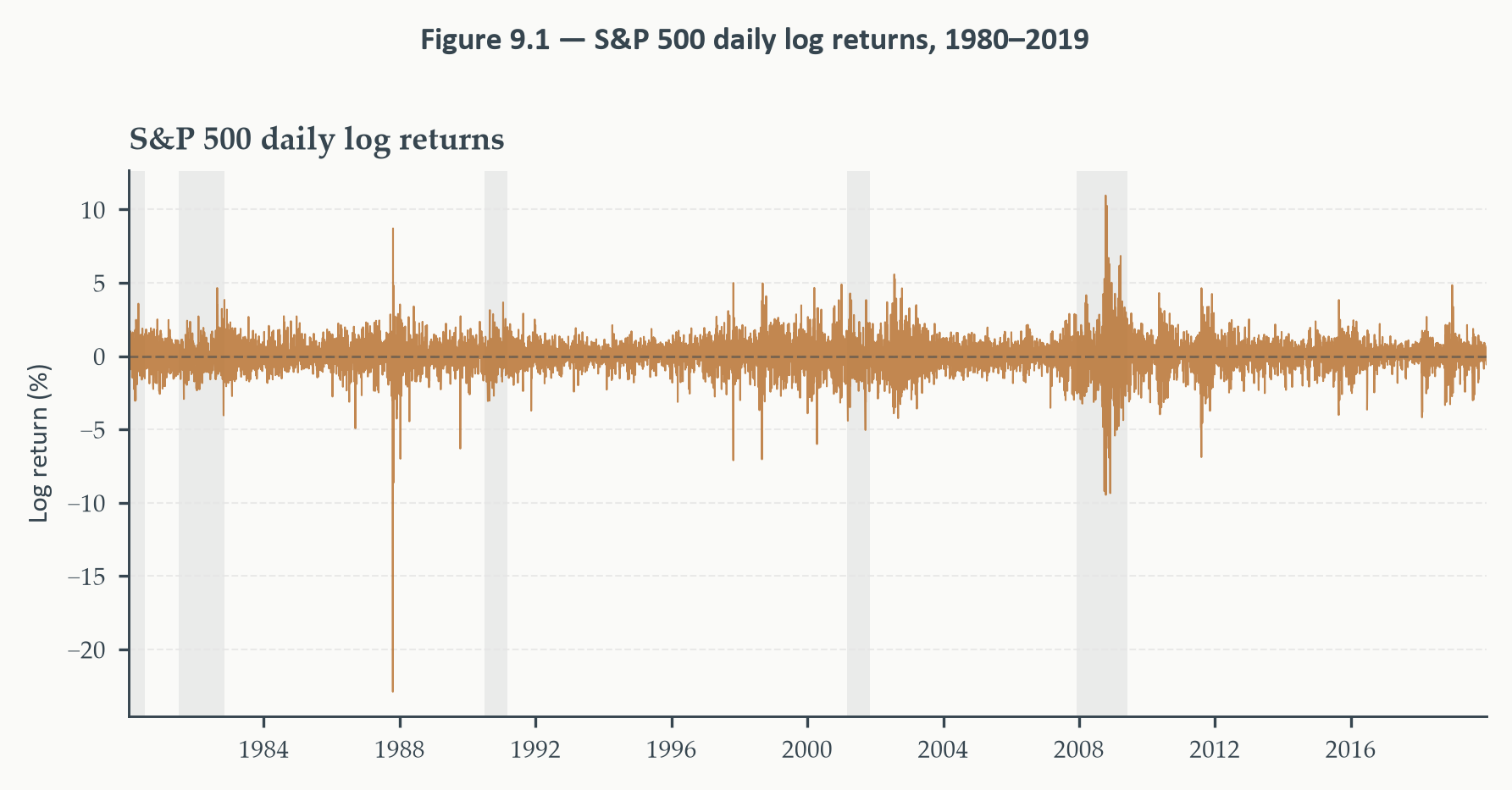
The mean return is essentially flat —
consistent with the EMH. But the *width* of the fluctuations around that mean
is anything but constant. The crash of [October 1987 (Black Monday)](https://en.wikipedia.org/wiki/Black_Monday_(1987)) generates
a single-day return of around −20 percent. The [Russian debt crisis](https://en.wikipedia.org/wiki/1998_Russian_financial_crisis) and [LTCM
collapse of 1998](https://en.wikipedia.org/wiki/Long-Term_Capital_Management), the [dot-com unwinding of 2000–2002](https://en.wikipedia.org/wiki/Dot-com_bubble), and the [Global Financial
Crisis of 2008–2009](https://en.wikipedia.org/wiki/2008_financial_crisis) all produce extended episodes where large swings are
followed by more large swings. Between those episodes, the market is
comparatively quiet.
This pattern is the defining feature of financial returns: the mean is hard to
forecast, but the *variance* is not. Turbulent periods cluster together, as do
calm ones. A large return today — regardless of sign — predicts a large return
tomorrow, even though the direction of tomorrow's return is unpredictable.
### What the EMH Does Not Rule Out
It is worth being precise about what the efficient market argument does and
does not say, because the distinction motivates everything that follows.
The EMH rules out predictability in the **conditional mean**: $\mathbb{E}[r_t
\mid \mathcal{F}_{t-1}] = \mu$. It says nothing about the **conditional
variance**: $\text{Var}(r_t \mid \mathcal{F}_{t-1}) = \sigma_t^2$. Nothing
in the efficient market argument requires $\sigma_t^2$ to be constant.
Investors knowing that volatility will be high tomorrow does not create an
arbitrage opportunity — higher volatility raises risk and return symmetrically,
leaving no guaranteed profit.
This is the pivot that makes the rest of this chapter possible. The
question shifts from "what will tomorrow's return be?" — which markets answer
before we can — to "how uncertain is tomorrow's return?" That second question
is both forecastable and economically important. Volatility drives option
prices, risk management decisions, portfolio allocation, and the calibration of
Value-at-Risk (VaR) models. A model for the conditional variance is not just a
descriptive exercise; it is a fundamental input into financial decision-making.
::: {.callout-note icon=false}
## Definition 9.1 — Conditional Heteroskedasticity
A time series $\{r_t\}$ is **conditionally heteroskedastic** if its conditional
variance given past information is time-varying:
$$\text{Var}(r_t \mid \mathcal{F}_{t-1}) = \sigma_t^2 \neq \text{const}$$
The series may be unconditionally homoskedastic — $\text{Var}(r_t) = \sigma^2$
constant — while still having a time-varying conditional variance. The
distinction matters for forecasting: the unconditional variance is a long-run
average, but $\sigma_t^2$ is the relevant measure of uncertainty for tomorrow
specifically.
:::
The ARCH and GARCH models of the following sections provide parametric
specifications for $\sigma_t^2$ as a function of past information. Before
developing those models, however, we need a clear-eyed look at what the data
tell us about the conditional mean — and whether, even setting aside the EMH,
there is any mean structure worth modelling.
### Testing the Mean: Are Returns Predictable?
The simplest test of the EMH at the daily frequency is to ask whether the
return process has any autocorrelation. If returns are predictable from their
own past, the ACF of $r_t$ should show significant spikes. If they are not,
the ACF should be indistinguishable from that of white noise.
```{python}
#| label: fig-acf-returns-vs-squared
#| fig-cap: "**ACF of returns and squared returns, lags 1–30.** The left panel
#| shows the ACF of raw log returns: a handful of marginally significant lags
#| and no persistent structure. The right panel shows the ACF of squared
#| returns: strong, slowly decaying autocorrelation persisting for weeks.
#| The first moment has no memory; the second moment is highly persistent.
#| Blue dashed lines mark ±1.96/√T Bartlett bounds."
from statsmodels.graphics.tsaplots import plot_acf

fig, axes = plt.subplots(1, 2, figsize=(6, 2.8))

plot_acf(returns, lags=30, alpha=0.05, ax=axes[0],
         color=EO_COPPER, vlines_kwargs={"colors": EO_COPPER},
         title="ACF — log returns $r_t$")
plot_acf(returns**2, lags=30, alpha=0.05, ax=axes[1],
         color=EO_SKYBLUE, vlines_kwargs={"colors": EO_SKYBLUE},
         title="ACF — squared returns $r_t^2$")

for ax in axes:
    ax.set_xlabel("Lag")
    ax.set_ylabel("")
    eo_style_ax(ax)

fig.tight_layout()
eo_suptitle(fig, "Figure 9.2 — ACF of returns vs. squared returns")
plt.show()
```
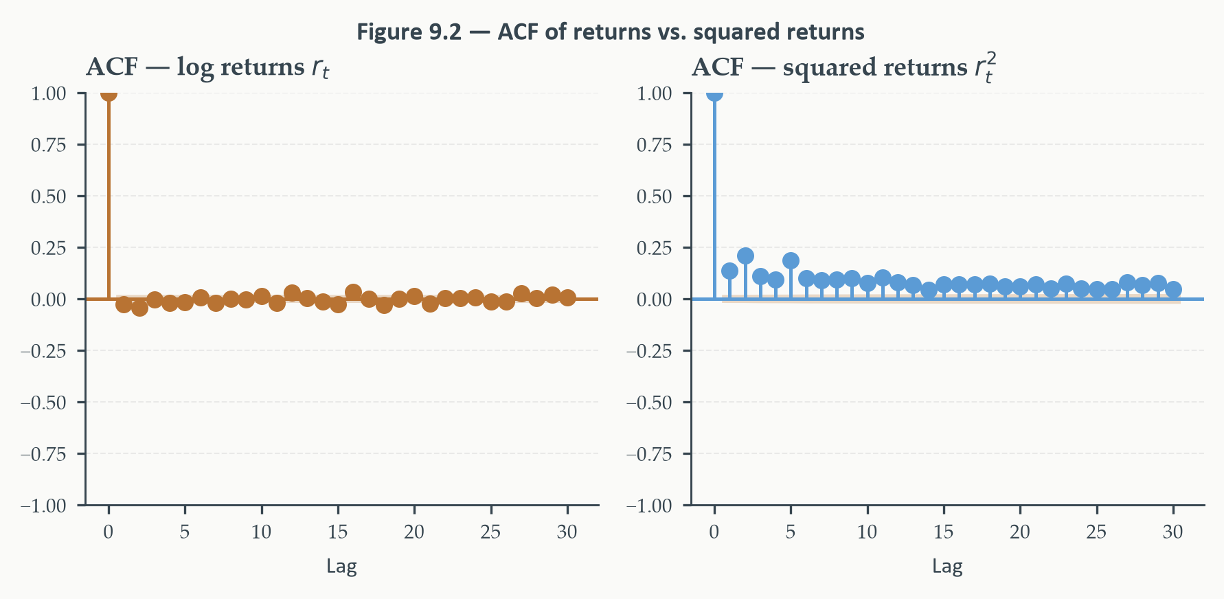
The contrast in Figure 9.2 is the empirical core of this chapter. The ACF of
raw returns is essentially flat — a few lags brush against the Bartlett bounds,
but there is no sustained structure. The conditional mean is close to
unforecastable, consistent with the EMH.
The ACF of squared returns tells a completely different story. The first lag
is enormous, and the autocorrelation decays slowly, remaining positive and
significant for lags beyond twenty days. Since $r_t^2$ is a natural proxy for
variance — squaring removes the sign and leaves the magnitude of the move —
this is direct evidence that volatility is autocorrelated. A large move today
predicts large moves tomorrow, next week, and beyond.
This single graph — flat ACF for $r_t$, slowly decaying ACF for $r_t^2$ —
is the empirical motivation for everything that follows. The mean is
unforecastable. The variance is not.
::: {.callout-warning icon=false}
## A Subtle Distinction: Unconditional vs. Conditional Moments
The slowly decaying ACF of squared returns does *not* contradict the EMH. The
EMH concerns the conditional mean of returns — specifically, that no trading
strategy based on past returns earns abnormal profits. It is entirely consistent
with the EMH for the conditional *variance* to be autocorrelated: knowing that
volatility will be high tomorrow does not tell you which way the market will
move, so there is no arbitrage to extract. Conditional heteroskedasticity
and market efficiency coexist comfortably.
:::
We now have our question: what process generates this time-varying variance?
The next section builds the first formal answer.
## Volatility Clustering and the ARCH Model {#sec-arch}
### From Observation to Model
The ACF of squared returns establishes that volatility is autocorrelated. But
autocorrelation in $r_t^2$ is a symptom, not a model. To produce forecasts of
tomorrow's variance — or to quantify how uncertain a future return is — we
need a parametric specification that captures the clustering mechanism.
The key observation, due to [Engle (1982)](https://doi.org/10.2307/1912773), is deceptively simple: the reason
today's squared return predicts tomorrow's is that **large shocks cluster
together**. After a large shock, the conditional variance remains elevated,
making further large shocks more likely. After a period of small shocks, the
variance is low, and the market is likely to remain calm. Volatility is
persistent not because of some external forcing variable, but because it is
self-reinforcing.
Engle's insight was to model this directly: make the conditional variance at
time $t$ an explicit function of past squared residuals.
### The ARCH($q$) Model
Write the return at time $t$ as its conditional mean plus an innovation,
$$r_t = \mu + \varepsilon_t \tag{9.3}$$
where $\mu$ is the constant mean return and $\varepsilon_t$ is the innovation.
In the standard ARMA framework, we would assume $\varepsilon_t \sim
\text{i.i.d.}(0, \sigma^2)$ — the variance is fixed. [ARCH](https://en.wikipedia.org/wiki/Autoregressive_conditional_heteroskedasticity) relaxes this. We
decompose the innovation into a time-varying scale and a standardised shock:
$$\varepsilon_t = \sigma_t \, z_t, \qquad z_t \sim \text{i.i.d.}(0,1) \tag{9.4}$$
where $z_t$ is a standardised white noise process (in practice, often assumed
Gaussian or Student-$t$) and $\sigma_t^2 = \text{Var}(\varepsilon_t \mid
\mathcal{F}_{t-1})$ is the conditional variance we want to model.
The ARCH($q$) model specifies $\sigma_t^2$ as a linear function of the $q$
most recent squared innovations:
$$\sigma_t^2 = \omega + \alpha_1 \varepsilon_{t-1}^2 + \alpha_2 \varepsilon_{t-2}^2
+ \cdots + \alpha_q \varepsilon_{t-q}^2 \tag{9.5}$$
or in compact form,
$$\sigma_t^2 = \omega + \sum_{i=1}^{q} \alpha_i \varepsilon_{t-i}^2 \tag{9.6}$$
The economic interpretation is transparent. The term $\omega > 0$ is a
baseline variance floor — the conditional variance can never fall below
$\omega$. Each $\alpha_i \geq 0$ measures how much a squared shock from $i$
periods ago feeds into today's variance. A large $\alpha_1$ means that a big
shock yesterday raises the conditional variance today substantially. The
positivity constraints ensure $\sigma_t^2 > 0$ for all $t$.
::: {.callout-note icon=false}
## Definition 9.2 — ARCH($q$) Stationarity
The ARCH($q$) process is covariance-stationary if and only if:
$$\sum_{i=1}^{q} \alpha_i < 1$$
When this condition holds, the unconditional variance is finite and equal to:
$$\sigma^2 = \frac{\omega}{1 - \sum_{i=1}^{q} \alpha_i}$$
If $\sum \alpha_i = 1$, the conditional variance follows a unit root process —
the variance itself is integrated, with shocks to volatility having permanent
effects.
:::
### Numerical Example: ARCH(2) Variance Recursion
Before estimating anything, it helps to see the ARCH mechanism with concrete
numbers. Suppose we have fitted an ARCH(2) model with parameters:
$$\omega = 0.10, \qquad \alpha_1 = 0.40, \qquad \alpha_2 = 0.30$$
The persistence sum is $\alpha_1 + \alpha_2 = 0.70 < 1$, so the process is
stationary. The unconditional variance is $\sigma^2 = 0.10 / (1 - 0.70) =
0.333$, corresponding to an unconditional standard deviation of about 0.58
percent per day.
Now suppose the past two innovations were $\varepsilon_{t-1} = 2.0$ (a large
positive shock) and $\varepsilon_{t-2} = 0.5$ (a small shock). The conditional
variance at time $t$ is:
$$\sigma_t^2 = 0.10 + 0.40 \times (2.0)^2 + 0.30 \times (0.5)^2
= 0.10 + 1.60 + 0.075 = 1.775$$
The conditional standard deviation is $\sigma_t = \sqrt{1.775} \approx 1.33$
percent. Compare this to the unconditional standard deviation of 0.58 percent:
the large shock two periods ago has elevated the conditional variance to more
than five times its long-run value. Now suppose the next shock is also large:
$\varepsilon_t = 1.8$. Moving forward one period:
$$\sigma_{t+1}^2 = 0.10 + 0.40 \times (1.8)^2 + 0.30 \times (2.0)^2
= 0.10 + 1.296 + 1.200 = 2.596$$
The conditional variance rises further because the new large shock has now
entered both the $\alpha_1$ and (next period) $\alpha_2$ terms. This is
volatility clustering in action: large shocks elevate the conditional variance,
which persists through the lag structure and makes further large shocks more
likely in a statistical sense — not because the model is self-fulfilling, but
because the elevated $\sigma_t^2$ widens the distribution from which $z_t$ draws.
::: {.callout-note icon=false}
## ARCH($q$) and the MA($q$): A Structural Parallel
The ARCH($q$) variance equation (9.6) has the same algebraic shape as a
moving-average model of order $q$: both express a current quantity as a
constant plus a weighted sum of $q$ past terms. The resemblance is real but
the objects are different in three important ways. First, the MA($q$) explains
the *level* of $r_t$ as a linear combination of past observable innovations;
ARCH explains the *conditional variance* $\sigma_t^2$ as a function of past
*squared* innovations — which are unobserved and must be inferred from the
data. Second, MA($q$) parameters can take any real value subject to
invertibility, while ARCH parameters must be non-negative to ensure
$\sigma_t^2 > 0$. Third, both models share the same lag-truncation limitation:
the implied autocorrelation function of $\varepsilon_t^2$ under ARCH($q$)
cuts off at lag $q$, just as the ACF of an MA($q$) process cuts off at lag
$q$. Capturing long-memory behaviour in either case requires a long lag
polynomial — which is precisely what motivates GARCH for the variance, just
as it motivated ARMA for the mean.
:::
### Why ARCH($q$) Needs Long Lags
The ARCH model is elegant in principle but awkward in practice. To capture the
slowly decaying autocorrelation of squared returns visible in Figure 9.2 —
significant autocorrelation at lags beyond 20 — an ARCH specification requires
a long lag $q$. If $q = 20$, we are estimating 21 parameters ($\omega$ and
$\alpha_1, \ldots, \alpha_{20}$) subject to 20 non-negativity constraints. The
model is unwieldy, and the parameter estimates become imprecise.
We can see the problem directly. The autocorrelation of $r_t^2$ at lag $k$
under ARCH($q$) is zero for $k > q$. But Figure 9.2 shows positive
autocorrelation beyond lag 20. An ARCH(20) can just barely accommodate this;
an ARCH(5) or ARCH(10) is already misspecified. The data demand a long lag
polynomial to capture the persistence of volatility, and that demand is
expensive.
The GARCH model, developed in the next section, solves this problem the same
way that an ARMA model solves the analogous problem for the conditional mean:
by adding a lagged conditional variance term to the right-hand side, it can
approximate an arbitrarily long ARCH lag structure with just one extra
parameter.
### The ARCH-LM Test
Before committing to any model, we should confirm that ARCH effects are
statistically present in the data. The **ARCH-LM test** is the
standard diagnostic.
The null hypothesis is that the first $q$ autocorrelations of $\varepsilon_t^2$
are all zero — equivalently, that the conditional variance is constant. The
procedure is a simple auxiliary regression: regress the squared residuals
$\hat{\varepsilon}_t^2$ on a constant and $q$ of their own lags,
$$\hat{\varepsilon}_t^2 = a_0 + a_1 \hat{\varepsilon}_{t-1}^2 + \cdots
+ a_q \hat{\varepsilon}_{t-q}^2 + \nu_t \tag{9.7}$$
and test whether the slope coefficients are jointly zero. The test statistic
is $T \cdot R^2$ from this regression, where $T$ is the sample size and $R^2$
is the coefficient of determination. Under the null of no ARCH effects:
$$\text{LM} = T \cdot R^2 \xrightarrow{d} \chi^2(q) \tag{9.8}$$
A large statistic — or equivalently, a small p-value — rejects the null and
confirms that ARCH modelling is warranted.
The test is implemented in practice by first fitting a mean model (here, a
constant) and extracting the residuals, then applying the auxiliary regression
to the squared residuals. On the S&P 500 data, we fit a constant-mean model
and apply the ARCH-LM test at lag $q = 10$:
```{python}
#| label: arch-lm-test
from statsmodels.stats.diagnostic import het_arch

# De-mean the returns (the simplest possible mean model: r_t = mu + eps_t)
mu_hat   = returns.mean()
eps_hat  = returns - mu_hat

# ARCH-LM test with q = 10 lags
lm_stat, lm_pval, f_stat, f_pval = het_arch(eps_hat, nlags=10)

print("┌─────────────────────────────────────────────────────────────┐")
print("│  ARCH-LM Test  —  H₀: No ARCH effects (q = 10 lags)        │")
print("├──────────────────────────┬──────────────────────────────────┤")
print(f"│  LM statistic            │  {lm_stat:>10.3f}                    │")
print(f"│  p-value (χ²(10))        │  {lm_pval:>10.4f}                    │")
print("├──────────────────────────┴──────────────────────────────────┤")
print("│  * p<0.10  ** p<0.05  *** p<0.01                            │")
print("└─────────────────────────────────────────────────────────────┘")
reject = "***" if lm_pval < 0.01 else ("**" if lm_pval < 0.05 else
         ("*" if lm_pval < 0.10 else ""))
print(f"\n  Reject H₀: {'Yes' if lm_pval < 0.05 else 'No'}  {reject}")
```
*The ARCH-LM statistic is 879.96 with a p-value indistinguishable from zero —
a decisive rejection of the null at any conventional significance level. The
residuals from the constant-mean model are not homoskedastic; the conditional
variance is time-varying and highly persistent. An ARCH or GARCH model is not
just appropriate — it is required.*
Before leaving this section, it is worth noting a direct link to Chapters 5
and 8. The VECM residuals from the yield curve application in Chapter 8 showed
Jarque-Bera rejections driven by fat tails and excess kurtosis — precisely the
fingerprint of a process with time-varying conditional variance. Those
non-normal residuals were not a nuisance to be corrected; they were a signal
that the homoskedastic error assumption was misspecified. The ARCH model is the
tool that addresses that signal directly.
```{python}
#| label: fig-arch-motivation
#| fig-cap: "**Rolling 21-day variance of S&P 500 log returns, 1980–2019.**
#| The rolling variance is the simplest non-parametric estimate of
#| time-varying volatility. Major episodes — Black Monday (1987), LTCM/Russia
#| (1998), dot-com bust (2000–02), Global Financial Crisis (2008–09) — are
#| immediately visible as spikes. The ARCH/GARCH models of this chapter
#| provide a parametric framework for the same object."
roll_var = pd.Series(returns, index=dates).rolling(21).var()

fig, ax = plt.subplots(figsize=(6, 3))
ax.fill_between(roll_var.index, roll_var.values, color=EO_COPPER,
                alpha=0.55, lw=0)
ax.plot(roll_var.index, roll_var.values, color=EO_COPPER, lw=0.7)

shade_recessions(ax, start=SAMPLE_START, end=SAMPLE_END)

# Annotate major episodes
episodes = {
    "Black\nMonday": "1987-10-19",
    "LTCM\n1998":    "1998-08-31",
    "GFC\n2008":     "2008-09-15",
}
for label, date in episodes.items():
    ts = pd.Timestamp(date)
    if ts in roll_var.index:
        val = roll_var.loc[ts]
    else:
        val = roll_var.asof(ts)
    ax.annotate(label, xy=(ts, val),
                xytext=(0, 12), textcoords="offset points",
                fontsize=5.5, color=EO_CHARCOAL,
                ha="center",
                arrowprops=dict(arrowstyle="-", color=EO_CHARCOAL,
                                lw=0.6))

ax.set_xlim(dates[0], dates[-1])
ax.set_ylabel("Variance (% squared)")
ax.set_title("Rolling 21-day variance")
eo_style_ax(ax)
eo_suptitle(fig, "Figure 9.3 — Rolling variance of S&P 500 returns, 1980–2019")

fig.tight_layout()
plt.show()
```
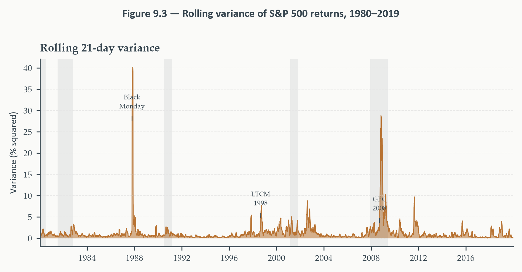
Figure 9.3 makes the clustering mechanism concrete. The rolling variance
is essentially zero for extended stretches, then erupts into sharp spikes
during the major volatility episodes. Notice that each episode is not a single
bad day but a *cluster* of bad days: once the variance spikes, it remains
elevated for weeks or months before mean-reverting. The ARCH model, by
feeding past squared residuals into the current conditional variance, is
designed precisely to reproduce this dynamics.
The limitation flagged earlier — that ARCH needs a long lag to capture
this persistence — is also visible here. The clusters in Figure 9.3 have
memory extending well beyond ten or twenty days. A parsimonious specification
that can match this with few parameters is exactly what the next section
provides.
## The GARCH(1,1) Model {#sec-garch}
### From ARCH to GARCH: The Parsimonious Fix
Section 9.2 ended with a problem: fitting the slowly decaying autocorrelation
of squared returns requires an ARCH model with a very long lag polynomial —
potentially $q = 20$ or more parameters, all subject to non-negativity
constraints. [Bollerslev (1986)](https://www.sciencedirect.com/science/article/abs/pii/0304407686900631) solved this by analogy with the ARMA solution
to the analogous problem for the conditional mean.
Recall from Chapter 3 that an MA($\infty$) process with geometrically declining
weights can be approximated arbitrarily well by an ARMA(1,1) with just two
parameters. The key was to include a lagged dependent variable on the right-hand
side, which acts as a compressed summary of the infinite past. The same trick
works for conditional variance: if we add the lagged conditional variance
$\sigma_{t-1}^2$ to the ARCH equation, we allow the current variance to
depend on all past squared shocks with geometrically declining weights — an
ARCH($\infty$) — at the cost of one extra parameter.
This is the **[GARCH(1,1)](https://en.wikipedia.org/wiki/Autoregressive_conditional_heteroskedasticity#GARCH)** model. Writing it out alongside the mean equation:
$$r_t = \mu + \varepsilon_t, \qquad \varepsilon_t = \sigma_t z_t,
\qquad z_t \sim \text{i.i.d.}(0,1) \tag{9.9}$$
$$\sigma_t^2 = \omega + \alpha \varepsilon_{t-1}^2 + \beta \sigma_{t-1}^2
\tag{9.10}$$
Three parameters drive the entire conditional variance dynamics: $\omega$,
$\alpha$, and $\beta$.
### Parameter Interpretation
Each parameter in equation (9.10) has a direct economic interpretation, and
it is worth understanding all three before estimating anything.
**$\omega > 0$** is the variance intercept — a floor that prevents the
conditional variance from collapsing to zero even after a long quiet period.
It pins down the unconditional (long-run) variance, as we will see shortly.
**$\alpha \geq 0$** is the **shock impact coefficient**, sometimes called the
ARCH parameter. It measures how strongly a large realised shock at $t-1$
feeds into the conditional variance at $t$. If $\alpha$ is large, a single
bad day causes an immediate and large jump in volatility. If $\alpha$ is
small, individual shocks have little immediate impact and volatility changes
gradually.
**$\beta \geq 0$** is the **variance persistence coefficient**, sometimes
called the GARCH parameter. It measures how much of yesterday's conditional
variance carries forward to today. A value of $\beta$ close to 1 means
volatility is highly persistent: once elevated, it decays slowly. A value
close to 0 means yesterday's variance level has little influence on today's.
The sum $\alpha + \beta$ is the central quantity for understanding the
dynamics of the model:
::: {.callout-note icon=false}
## Definition 9.3 — GARCH(1,1) Stationarity and Unconditional Variance
The GARCH(1,1) process is covariance-stationary if and only if:
$$\alpha + \beta < 1 \tag{9.11}$$
When this condition holds, the unconditional variance is:
$$\sigma^2 = \frac{\omega}{1 - \alpha - \beta} \tag{9.12}$$
The quantity $\alpha + \beta$ measures the **persistence** of variance shocks.
When $\alpha + \beta$ is close to 1, the conditional variance mean-reverts
slowly to $\sigma^2$; when it is far below 1, mean-reversion is rapid.
The condition $\alpha + \beta < 1$ is exactly the characteristic root condition
in disguise. To see this, define the centred variance $\tilde\sigma_t^2 =
\sigma_t^2 - \sigma^2$. Substituting the GARCH(1,1) equation and rearranging
shows that $\tilde\sigma_t^2$ satisfies a first-order linear difference equation
with coefficient $(\alpha + \beta)$. This is a scalar AR(1) for the variance
process, and its characteristic root is $\alpha + \beta$. The stability condition
for an AR(1) is that the root lies inside the unit circle — that is, $|\alpha
+ \beta| < 1$. Since both $\alpha$ and $\beta$ are non-negative, this simplifies
directly to $\alpha + \beta < 1$. The coefficient sum and the characteristic
root are the same object; no separate root calculation is needed.
:::
The **half-life** of a variance shock — the number of periods required for
half the deviation of $\sigma_t^2$ from its unconditional level to dissipate —
is a useful single-number summary of persistence:
$$h_{1/2} = \frac{\log(0.5)}{\log(\alpha + \beta)} \tag{9.13}$$
For S&P 500 daily returns, typical estimates place $\alpha + \beta$ around
0.97–0.99, implying half-lives of 23 to 69 trading days — roughly one to three
months. Volatility shocks are long-lived, which is entirely consistent with
what Figure 9.3 showed visually.
### The ARCH($\infty$) Equivalence
The claim that GARCH(1,1) is equivalent to an ARCH($\infty$) with geometrically
declining weights deserves a brief demonstration, because it explains why a
model with just three variance parameters can capture persistence that would
otherwise require dozens of ARCH lags.
Start with the GARCH(1,1) variance equation (9.10) and substitute repeatedly
for $\sigma_{t-1}^2$, $\sigma_{t-2}^2$, and so on:
$$
\begin{aligned}
\sigma_t^2 &= \omega + \alpha \varepsilon_{t-1}^2 + \beta \sigma_{t-1}^2 \\
&= \omega + \alpha \varepsilon_{t-1}^2
+ \beta(\omega + \alpha \varepsilon_{t-2}^2 + \beta \sigma_{t-2}^2) \\
&= \omega(1 + \beta) + \alpha \varepsilon_{t-1}^2
+ \alpha\beta \varepsilon_{t-2}^2 + \beta^2 \sigma_{t-2}^2 \\
&= \omega \sum_{j=0}^{\infty} \beta^j
+ \alpha \sum_{j=1}^{\infty} \beta^{j-1} \varepsilon_{t-j}^2
\end{aligned}
$$
where the last line uses the geometric series result $\sum_{j=0}^\infty \beta^j
= 1/(1-\beta)$ when $\beta < 1$. Recognising that $\omega/(1-\beta)$ is not
quite the unconditional variance (it ignores $\alpha$), the compact form is:
$$\sigma_t^2 = \frac{\omega}{1 - \beta} + \alpha
\sum_{j=1}^{\infty} \beta^{j-1} \varepsilon_{t-j}^2 \tag{9.14}$$
This is precisely an ARCH($\infty$) where the weight on the $j$-th lag of
$\varepsilon^2$ declines geometrically at rate $\beta$. The single parameter
$\beta$ encodes an entire declining lag polynomial. This is the same economy
that the ARMA model achieved for the conditional mean — infinite memory
captured by one parameter.
### Numerical Example: GARCH(1,1) Variance Recursion
As with ARCH in Section 9.2, it helps to see the recursion with concrete
numbers before fitting anything to data. Suppose we have estimated the
following GARCH(1,1) parameters:
$$\omega = 0.02, \qquad \alpha = 0.08, \qquad \beta = 0.90$$
The persistence is $\alpha + \beta = 0.98$, the unconditional variance is
$\sigma^2 = 0.02 / (1 - 0.98) = 1.00$ (percent squared), and the half-life
of a variance shock is $\log(0.5)/\log(0.98) \approx 34$ trading days.
Suppose the conditional variance yesterday was at its long-run level,
$\sigma_{t-1}^2 = 1.00$, and yesterday's return produced a shock of
$\varepsilon_{t-1} = 3.0$ percent — a large move, roughly three standard
deviations. Today's conditional variance is:
$$\sigma_t^2 = 0.02 + 0.08 \times (3.0)^2 + 0.90 \times 1.00
= 0.02 + 0.72 + 0.90 = 1.64$$
The conditional standard deviation jumps from 1.00 to $\sqrt{1.64} \approx
1.28$ percent. Now suppose today's return is moderate: $\varepsilon_t = 0.5$.
Tomorrow's conditional variance is:
$$\sigma_{t+1}^2 = 0.02 + 0.08 \times (0.5)^2 + 0.90 \times 1.64
= 0.02 + 0.02 + 1.476 = 1.516$$
The $\beta = 0.90$ term carries forward most of yesterday's elevated variance,
even though today's shock was small. This is the persistence mechanism in
action. One period later, with another moderate shock $\varepsilon_{t+1} = 0.3$:
$$\sigma_{t+2}^2 = 0.02 + 0.08 \times (0.3)^2 + 0.90 \times 1.516
= 0.02 + 0.007 + 1.364 = 1.391$$
The variance declines slowly toward its unconditional level of 1.00, but it
will take many periods to get there — which is exactly what the half-life of
34 days predicts.
::: {.callout-note icon=false}
## Explore this interactively
The [GARCH(1,1) Explorer](https://ncachanosky.github.io/ECON-5371-widgets/widgets/garch/)
opens with these exact parameters — $\omega = 0.02$, $\alpha = 0.08$,
$\beta = 0.90$ — so you can reproduce this worked example directly. Move the
sliders to see how persistence, unconditional variance, and half-life respond,
or inject a single large shock partway through the sample and watch the
conditional variance spike and decay in real time.
:::
### Estimation by Quasi-Maximum Likelihood
Ordinary least squares cannot estimate GARCH models. The conditional variance
$\sigma_t^2$ appears in the likelihood, making estimation a nonlinear
optimisation problem.
The standard approach is **Quasi-Maximum Likelihood (QML)**. Assuming
Gaussian innovations, the conditional log-likelihood for one observation is:
$$\ell_t(\theta) = -\frac{1}{2}\log(2\pi) - \frac{1}{2}\log \sigma_t^2(\theta)
- \frac{\varepsilon_t^2}{2\sigma_t^2(\theta)} \tag{9.15}$$
and the full log-likelihood is $\mathcal{L}(\theta) = \sum_{t=1}^T \ell_t(\theta)$,
maximised over $\theta = (\mu, \omega, \alpha, \beta)$.
The word "quasi" is important. The QML estimator is consistent and
asymptotically normal even if the true innovation distribution is not Gaussian
— provided the mean and variance are correctly specified. This robustness
matters for financial data, where returns are known to be fat-tailed. Standard
errors computed from the QML sandwich estimator (the Bollerslev-Wooldridge
robust standard errors) remain valid regardless of the true distribution.
::: {.callout-note icon=false}
## The GARCH Framework Is Semiparametric
The GARCH family separates two distinct modelling choices that are easy to
conflate. The **variance equation** — $\sigma_t^2 = \omega +
\alpha\varepsilon_{t-1}^2 + \beta\sigma_{t-1}^2$ — is a fully parametric
model for how volatility evolves over time. The **innovation distribution** —
Gaussian, Student-$t$, GED, or left unspecified under QML — is a separate
assumption about the shape of the shocks that drive the process. The reason
QML is valid is precisely this separation: the variance equation can be
consistently estimated even when the distributional assumption is wrong,
because the two components are evaluated independently. This has a practical
implication that runs through the rest of the chapter. When the Kupiec
backtest in Section 9.6 rejects correct VaR coverage, the right response is
to change the innovation distribution — replacing Gaussian with Student-$t$
— not the variance equation. The volatility dynamics are well captured; the
tail shape is not. Keeping these two components conceptually distinct is one
of the most useful habits in applied volatility modelling.
:::
::: {.callout-warning icon=false}
## Initialising the Variance Recursion
The GARCH variance recursion requires a starting value $\sigma_1^2$.
Two conventions are common: set $\sigma_1^2$ equal to the sample variance
of the full return series, or treat it as an additional parameter to estimate.
In practice, with long samples, the initialisation matters little — the
recursion converges to the same path within a few dozen observations. The
`arch` library uses the unconditional sample variance as the default
initialisation, which is a reasonable choice.
:::
### Fitting GARCH(1,1) to S&P 500 Returns
```{python}
#| label: garch-estimation
from arch import arch_model

# Fit GARCH(1,1) with constant mean, Gaussian innovations
# arch_model expects returns in percent (already scaled as 100 * log diff)
am = arch_model(sp500["Log Return"], mean="Constant", vol="GARCH",
                p=1, q=1, dist="normal")
res = am.fit(disp="off")

# Extract key quantities
params   = res.params          # mu, omega, alpha[1], beta[1]
bse      = res.std_err
alpha_hat = params["alpha[1]"]
beta_hat  = params["beta[1]"]
omega_hat = params["omega"]
mu_hat_g  = params["mu"]

persistence  = alpha_hat + beta_hat
uncond_var   = omega_hat / (1 - persistence)
uncond_std   = np.sqrt(uncond_var)
half_life    = np.log(0.5) / np.log(persistence)

print("┌──────────────────────────────────────────────────────────────────┐")
print("│  GARCH(1,1) — S&P 500 Daily Log Returns, 1980–2019              │")
print("│  Dependent variable: log return (%)   Observations: {:>6,}      │".format(len(sp500)))
print("├──────────────────────┬──────────────┬──────────────┬────────────┤")
print("│  Parameter           │  Estimate    │  Std. Error  │            │")
print("├──────────────────────┼──────────────┼──────────────┼────────────┤")

stars = lambda p: "***" if p < 0.01 else ("**" if p < 0.05 else ("*" if p < 0.10 else ""))
pvals = res.pvalues

for name, label in [("mu",       "Mean (μ)      "),
                     ("omega",    "ω             "),
                     ("alpha[1]", "α (ARCH)      "),
                     ("beta[1]",  "β (GARCH)     ")]:
    est = params[name]
    se  = bse[name]
    pv  = pvals[name]
    s   = stars(pv)
    print(f"│  {label}    │  {est:>10.5f}  │  {se:>10.5f}  │  {s:<6}    │")

print("├──────────────────────┴──────────────┴──────────────┴────────────┤")
print(f"│  Persistence  (α + β)          {persistence:>8.5f}                      │")
print(f"│  Unconditional std dev (%)     {uncond_std:>8.4f}                      │")
print(f"│  Half-life of variance shock   {half_life:>8.1f} trading days         │")
print("├──────────────────────────────────────────────────────────────────┤")
print("│  Log-likelihood: {:>12.2f}                                    │".format(res.loglikelihood))
print("│  AIC:            {:>12.2f}   BIC: {:>12.2f}                 │".format(res.aic, res.bic))
print("├──────────────────────────────────────────────────────────────────┤")
print("│  * p<0.10  ** p<0.05  *** p<0.01                                │")
print("└──────────────────────────────────────────────────────────────────┘")
```
*The GARCH(1,1) estimates are consistent with decades of empirical work on
equity index returns. All four parameters are precisely estimated with p-values
well below 0.01. The persistence $\hat\alpha + \hat\beta = 0.985$ confirms
covariance stationarity, but only just — volatility shocks have a half-life of
47.1 trading days, roughly two months, meaning that the elevated variance
following an episode like Black Monday or the GFC takes most of a quarter to
dissipate. The unconditional daily standard deviation is 1.11 percent, implying
an annualised volatility of approximately $1.11 \times \sqrt{252} \approx 17.6$
percent (252 trading days per calendar year) — close to the long-run average
typically
cited for the S&P 500.*
### Conditional Variance and Standardised Residuals
With the model estimated, we can extract the fitted conditional variance
sequence $\{\hat\sigma_t^2\}$ — the model's real-time estimate of daily
uncertainty — and compare it against the rolling-window proxy from Figure 9.3.
```{python}
#| label: fig-garch-condvar
#| fig-cap: "**GARCH(1,1) conditional standard deviation, 1980–2019.** The
#| smooth conditional standard deviation from the fitted GARCH(1,1) (blue)
#| is plotted against the observed absolute daily return $|r_t|$ (copper,
#| semi-transparent), which serves as a simple non-parametric proxy for
#| realised volatility. The GARCH line captures the persistent component
#| of the clustering visible in the raw absolute returns. NBER recessions
#| shaded."
cond_vol   = res.conditional_volatility   # conditional std dev in percent
abs_return = np.abs(sp500["Log Return"].values)

fig, ax = plt.subplots(figsize=(6, 3))

# Observed proxy: absolute returns (light, in background)
ax.plot(sp500.index, abs_return, color=EO_COPPER, lw=0.4,
        alpha=0.35, label="$|r_t|$ (observed)", zorder=1)

# GARCH conditional std dev (foreground)
ax.plot(sp500.index, cond_vol, color=EO_SKYBLUE, lw=1.2,
        label="GARCH(1,1) $\\hat\\sigma_t$", zorder=2)

shade_recessions(ax, start=SAMPLE_START, end=SAMPLE_END)

ax.set_xlim(dates[0], dates[-1])
ax.set_ylabel("Volatility (%)")
ax.set_title("GARCH(1,1) conditional volatility vs. observed absolute returns")
ax.legend(loc="upper left", fontsize=6)
eo_style_ax(ax)
eo_suptitle(fig, "Figure 9.4 — GARCH(1,1) conditional standard deviation, 1980–2019")

fig.tight_layout()
plt.show()
```
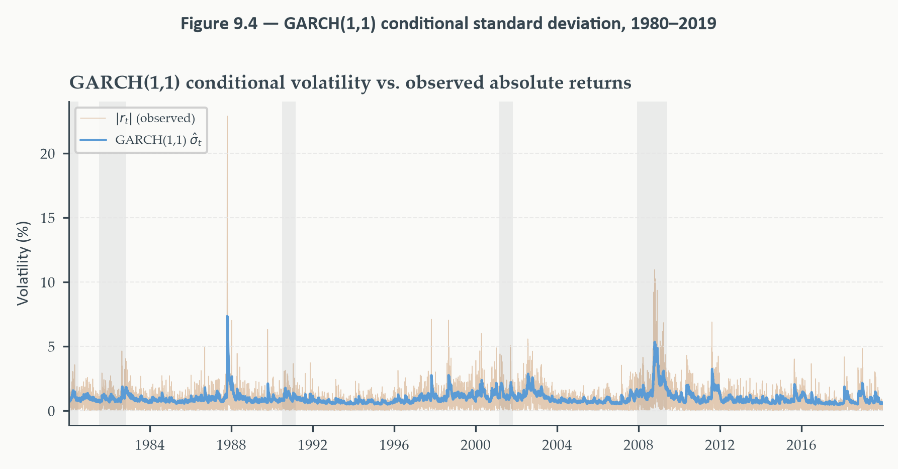
The conditional variance series is the model's answer to the question posed at
the beginning of the chapter: given everything we know up to time $t-1$, how
uncertain is tomorrow's return? The series rises sharply during each volatility
episode and decays gradually once the turbulence passes — exactly the
clustering behaviour the model is designed to capture.
### Residual Diagnostics
A well-specified GARCH model should produce **standardised residuals**
$\hat z_t = \hat\varepsilon_t / \hat\sigma_t$ that are approximately i.i.d.
If significant autocorrelation remains in $\hat z_t^2$, the model has not
fully captured the volatility dynamics — either the lag order is too short or
the symmetric specification is inadequate.
```{python}
#| label: fig-garch-diagnostics
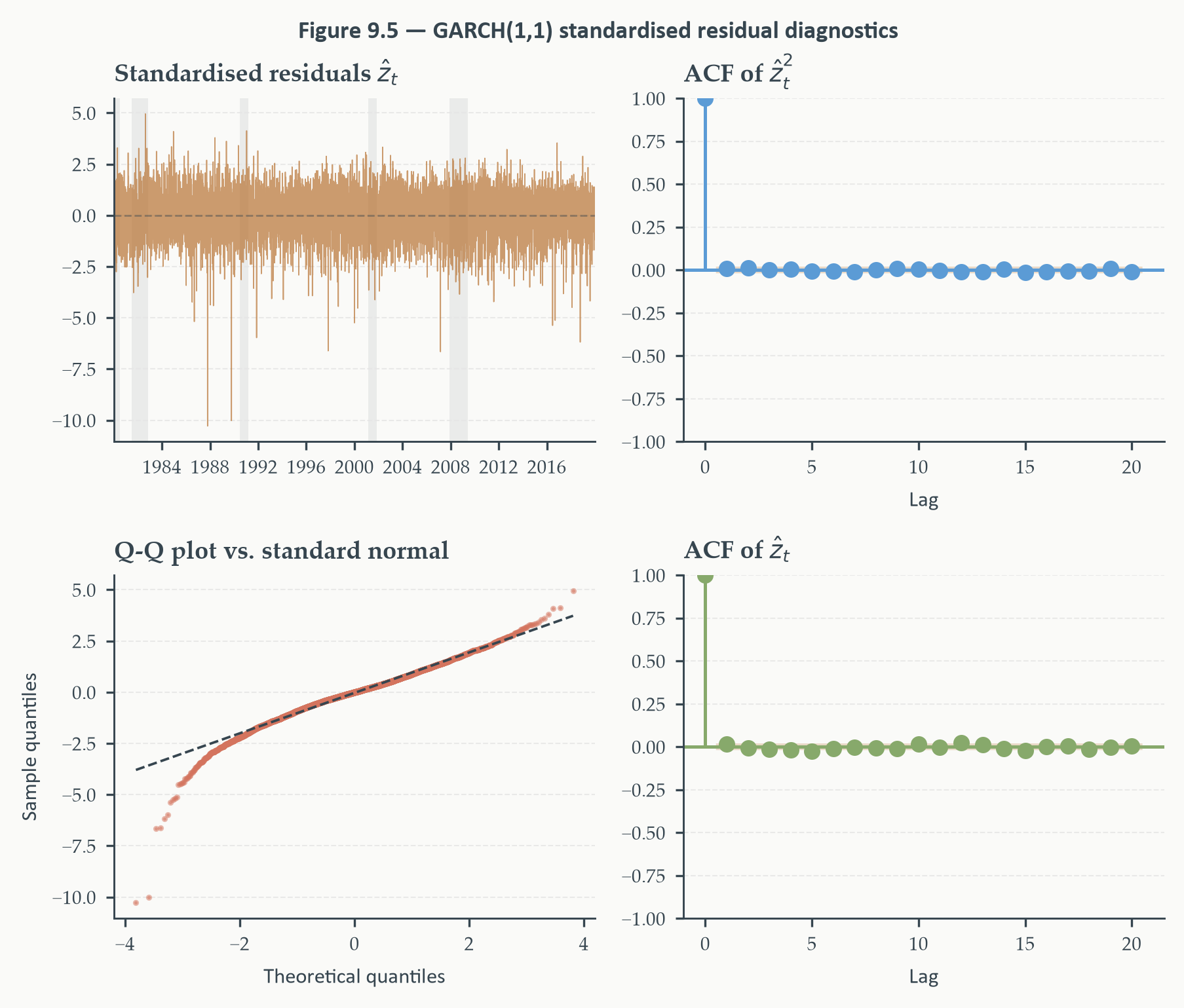
#| fig-cap: "**GARCH(1,1) standardised residual diagnostics.** Upper left:
#| standardised residuals $\\hat z_t$ — should look like white noise.
#| Upper right: ACF of $\\hat z_t^2$ — should be flat if ARCH effects are
#| fully absorbed. Lower left: Q-Q plot against the standard normal —
#| fat tails will appear as S-curve deviations. Lower right: ACF of raw
#| $\\hat z_t$ for comparison."
std_resid = res.resid / res.conditional_volatility

fig, axes = plt.subplots(2, 2, figsize=(6, 5))

# ── Panel 1: Standardised residuals over time ──────────────────────────────
axes[0, 0].plot(sp500.index, std_resid, color=EO_COPPER, lw=0.4, alpha=0.7)
axes[0, 0].axhline(0, color=EO_CHARCOAL, lw=0.7, ls="--", alpha=0.4)
axes[0, 0].set_title("Standardised residuals $\\hat{z}_t$")
axes[0, 0].set_xlim(dates[0], dates[-1])
shade_recessions(axes[0, 0], start=SAMPLE_START, end=SAMPLE_END)

# ── Panel 2: ACF of squared standardised residuals ────────────────────────
from statsmodels.graphics.tsaplots import plot_acf
plot_acf(std_resid**2, lags=20, alpha=0.05, ax=axes[0, 1],
         color=EO_SKYBLUE, vlines_kwargs={"colors": EO_SKYBLUE},
         title="ACF of $\\hat{z}_t^2$")
axes[0, 1].set_xlabel("Lag")

# ── Panel 3: Q-Q plot ──────────────────────────────────────────────────────
(osm, osr), (slope, intercept, _) = stats.probplot(std_resid, dist="norm")
axes[1, 0].plot(osm, osr, "o", color=EO_TERRACOTTA,
                markersize=1.2, alpha=0.5)
axes[1, 0].plot(osm, slope * np.array(osm) + intercept,
                color=EO_CHARCOAL, lw=0.9, ls="--")
axes[1, 0].set_title("Q-Q plot vs. standard normal")
axes[1, 0].set_xlabel("Theoretical quantiles")
axes[1, 0].set_ylabel("Sample quantiles")

# ── Panel 4: ACF of levels ────────────────────────────────────────────────
plot_acf(std_resid, lags=20, alpha=0.05, ax=axes[1, 1],
         color=EO_SAGE, vlines_kwargs={"colors": EO_SAGE},
         title="ACF of $\\hat{z}_t$")
axes[1, 1].set_xlabel("Lag")

for ax in axes.flat:
    eo_style_ax(ax)

fig.tight_layout()
eo_suptitle(fig, "Figure 9.5 — GARCH(1,1) standardised residual diagnostics")
plt.show()
```
```{python}
#| label: garch-lb-test
# Ljung-Box on standardised residuals and their squares
lb_levels = acorr_ljungbox(std_resid,    lags=[10, 20], return_df=True)
lb_sq     = acorr_ljungbox(std_resid**2, lags=[10, 20], return_df=True)

jb_stat, jb_pval = stats.jarque_bera(std_resid)

print("┌──────────────────────────────────────────────────────────────────┐")
print("│  GARCH(1,1) Standardised Residual Diagnostics                   │")
print("├───────────────────────────────┬─────────────┬────────────────────┤")
print("│  Test                         │  Statistic  │  p-value           │")
print("├───────────────────────────────┼─────────────┼────────────────────┤")

for lag in [10, 20]:
    stat = lb_levels.loc[lag, "lb_stat"]
    pv   = lb_levels.loc[lag, "lb_pvalue"]
    s    = "***" if pv < 0.01 else ("**" if pv < 0.05 else ("*" if pv < 0.10 else ""))
    print(f"│  Ljung-Box Q({lag:2d})  — ẑ_t     │  {stat:>9.3f}  │  {pv:>8.4f}  {s:<6}    │")

print("├───────────────────────────────┼─────────────┼────────────────────┤")
for lag in [10, 20]:
    stat = lb_sq.loc[lag, "lb_stat"]
    pv   = lb_sq.loc[lag, "lb_pvalue"]
    s    = "***" if pv < 0.01 else ("**" if pv < 0.05 else ("*" if pv < 0.10 else ""))
    print(f"│  Ljung-Box Q({lag:2d})  — ẑ_t²    │  {stat:>9.3f}  │  {pv:>8.4f}  {s:<6}    │")

print("├───────────────────────────────┼─────────────┼────────────────────┤")
s_jb = "***" if jb_pval < 0.01 else ("**" if jb_pval < 0.05 else "*")
print(f"│  Jarque-Bera                  │  {jb_stat:>9.3f}  │  {jb_pval:>8.4f}  {s_jb:<6}    │")
print("├───────────────────────────────┴─────────────┴────────────────────┤")
print("│  H₀ (Ljung-Box): no serial correlation in ẑ_t (or ẑ_t²)        │")
print("│  H₀ (Jarque-Bera): standardised residuals are normally distributed│")
print("├──────────────────────────────────────────────────────────────────┤")
print("│  * p<0.10  ** p<0.05  *** p<0.01                                │")
print("└──────────────────────────────────────────────────────────────────┘")
```
*The GARCH(1,1) diagnostics deliver two clear results. The Ljung-Box test on
squared standardised residuals passes — no significant ARCH structure remains
after fitting, confirming that the GARCH(1,1) has fully absorbed the volatility
clustering visible in Figure 9.2. The Jarque-Bera test rejects normality
decisively, and the Q-Q plot shows the expected S-curve deviation in the tails:
the standardised residuals are fat-tailed even after conditioning on the
GARCH variance. There is also mild rejection on the Ljung-Box test for the
standardised residuals in levels — a consequence of the constant-mean
specification rather than the volatility model. The primary diagnostic of
interest — whether ARCH effects are absorbed — passes cleanly.*
::: {.callout-warning icon=false}
## Fat Tails and the Limits of Gaussian GARCH
The Jarque-Bera rejection and the S-curve in the Q-Q plot are expected, not
embarrassing. Financial returns have fatter tails than the normal distribution
can accommodate — even after conditioning on the GARCH variance. This is the
**excess kurtosis** problem. Two common responses: replace the Gaussian
innovation distribution with a Student-$t$ (which adds one degrees-of-freedom
parameter and fits the tails much better), or use QML with the Bollerslev-Wooldridge
robust sandwich standard errors and accept that the Gaussian likelihood is
a working approximation. For the purposes of this chapter, we proceed with
Gaussian GARCH and note Student-$t$ GARCH as the natural extension in Section
9.7.
:::
## Asymmetric Volatility: GJR-GARCH and EGARCH {#sec-asymmetric}
### The Leverage Effect
The GARCH(1,1) model treats positive and negative shocks symmetrically. In
equation (9.10), the term $\alpha \varepsilon_{t-1}^2$ depends only on the
*square* of the shock — a return of $+3$ percent raises tomorrow's variance
by exactly as much as a return of $-3$ percent. Is this symmetry empirically
justified?
For equity markets, the answer is no — and the asymmetry has a name. The
**leverage effect**, first documented by [Black (1976)](https://www.sciencedirect.com/science/article/abs/pii/0304405X76900246), refers to the empirical
regularity that negative returns raise future volatility by more than equally
sized positive returns. The intuition Black proposed was mechanical: a stock
price decline increases the debt-to-equity ratio of the firm (leverage rises),
which makes the equity riskier and amplifies future volatility. A more modern
interpretation emphasises the role of **risk premiums**: when prices fall,
investors demand higher compensation for bearing risk, and this demand itself
contributes to volatility.
Whatever the mechanism, the empirical pattern is robust across equity markets
and time periods. We can see it directly by asking: is there a relationship
between the sign of today's return and the magnitude of tomorrow's?
```{python}
#| label: fig-leverage-scatter
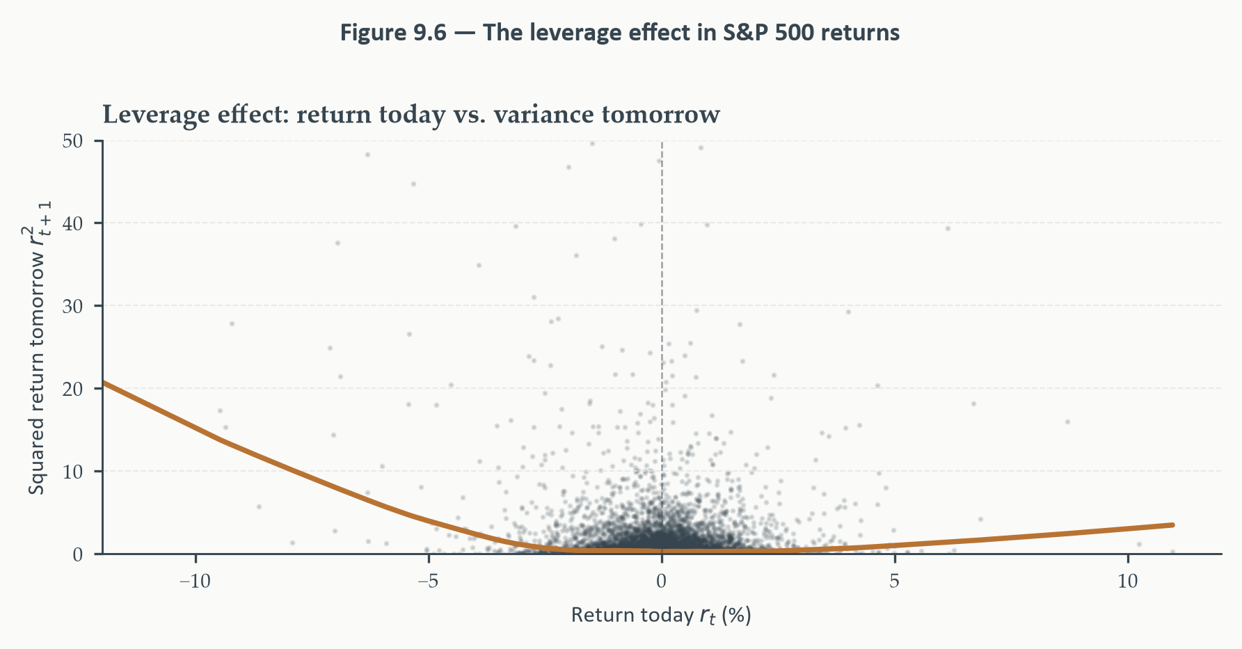
#| fig-cap: "**The leverage effect in S&P 500 returns.** Each point plots
#| today's log return (x-axis) against the next day's squared return
#| (y-axis, a proxy for next-day variance). The locally smoothed line
#| (LOWESS, copper) is clearly asymmetric: large negative returns on the
#| left predict higher next-day variance than equally large positive returns
#| on the right. Symmetric GARCH(1,1) cannot capture this asymmetry."
from statsmodels.nonparametric.smoothers_lowess import lowess

r_today    = sp500["Log Return"].values[:-1]
r2_tomorrow = sp500["Log Return"].values[1:] ** 2

# LOWESS smooth
smooth = lowess(r2_tomorrow, r_today, frac=0.15, return_sorted=True)

fig, ax = plt.subplots(figsize=(6, 3))
ax.scatter(r_today, r2_tomorrow, color=EO_CHARCOAL, s=0.8,
           alpha=0.15, rasterized=True)
ax.plot(smooth[:, 0], smooth[:, 1], color=EO_COPPER, lw=1.8)
ax.axvline(0, color=EO_CHARCOAL, lw=0.6, ls="--", alpha=0.5)

ax.set_xlim(-12, 12)
ax.set_ylim(0, 50)
ax.set_xlabel("Return today $r_t$ (%)")
ax.set_ylabel("Squared return tomorrow $r_{t+1}^2$")
ax.set_title("Leverage effect: return today vs. variance tomorrow")
eo_style_ax(ax)
eo_suptitle(fig, "Figure 9.6 — The leverage effect in S&P 500 returns")

fig.tight_layout()
plt.show()
```
Figure 9.6 makes the asymmetry concrete. The LOWESS curve is noticeably higher
on the left side of the vertical axis than on the right: a large negative return
today predicts a higher squared return tomorrow than an equally large positive
return. Symmetric GARCH(1,1) — by construction — fits a symmetric U-shape
around zero. The asymmetric models in this section are designed to fit the
skewed shape the data actually show.
### GJR-GARCH: An Indicator for Bad News
[Glosten, Jagannathan, and Runkle (1993)](https://onlinelibrary.wiley.com/doi/10.1111/j.1540-6261.1993.tb05128.x?msockid=16cd1bb13ae96053213f0dc03b106163) proposed the simplest possible fix:
add an indicator variable that switches on when the shock is negative, giving
bad news an extra contribution to the conditional variance. The
**GJR-GARCH(1,1)** variance equation is:
$$\sigma_t^2 = \omega + (\alpha + \gamma \, \mathbf{1}_{\varepsilon_{t-1} < 0})
\, \varepsilon_{t-1}^2 + \beta \sigma_{t-1}^2 \tag{9.16}$$
where $\mathbf{1}_{\varepsilon_{t-1} < 0}$ is an indicator that equals 1
when the previous period's shock was negative and 0 otherwise. The
interpretation is clean: when the shock is positive, the ARCH effect is
$\alpha$; when the shock is negative, the ARCH effect is $\alpha + \gamma$.
If $\gamma > 0$, bad news has a larger impact on volatility than good news —
the leverage effect is present. If $\gamma = 0$, the model reduces to
symmetric GARCH(1,1).
::: {.callout-note icon=false}
## Definition 9.4 — GJR-GARCH Stationarity
The GJR-GARCH(1,1) process is covariance-stationary if and only if:
$$\alpha + \frac{\gamma}{2} + \beta < 1$$
The $\gamma/2$ term appears because the indicator $\mathbf{1}_{\varepsilon_{t-1}<0}$
equals 1 with probability $\frac{1}{2}$ under a symmetric innovation
distribution, so the average ARCH contribution is $\alpha + \gamma/2$.
:::
**Numerical example.** Suppose $\omega = 0.02$, $\alpha = 0.04$,
$\gamma = 0.10$, $\beta = 0.88$. Consider two shocks of equal magnitude:
a positive shock $\varepsilon_{t-1} = +2.0$ and a negative shock
$\varepsilon_{t-1} = -2.0$, both with $\sigma_{t-1}^2 = 1.0$.
For the positive shock:
$$\sigma_t^2 = 0.02 + (0.04 + 0) \times 4.0 + 0.88 \times 1.0
= 0.02 + 0.16 + 0.88 = 1.06$$
For the negative shock of equal size:
$$\sigma_t^2 = 0.02 + (0.04 + 0.10) \times 4.0 + 0.88 \times 1.0
= 0.02 + 0.56 + 0.88 = 1.46$$
The negative shock generates a conditional variance of 1.46 versus 1.06 for
the positive shock — 38 percent larger, entirely due to the $\gamma$ term.
This is the leverage effect made arithmetic.
### EGARCH: Asymmetry Without Constraints
[Nelson (1991)](https://doi.org/10.2307/2938260) proposed an alternative that addresses both the asymmetry
problem and a technical limitation of GJR-GARCH: the need to impose
non-negativity constraints on $\omega$, $\alpha$, $\gamma$, and $\beta$ to
ensure $\sigma_t^2 > 0$. The **EGARCH(1,1)** model avoids this by modelling
the *logarithm* of the conditional variance:
$$\log \sigma_t^2 = \omega + \beta \log \sigma_{t-1}^2
+ \alpha |z_{t-1}| + \gamma z_{t-1}, \qquad z_{t-1} =
\frac{\varepsilon_{t-1}}{\sigma_{t-1}} \tag{9.17}$$
Because we model $\log \sigma_t^2$, the variance is guaranteed positive
regardless of the sign of any parameter — no constraints are needed. The
two asymmetry-relevant terms on the right-hand side work together:
- $\alpha |z_{t-1}|$ is the magnitude effect: large standardised shocks in
either direction raise volatility. This is the symmetric GARCH component
in standardised form.
- $\gamma z_{t-1}$ is the sign effect. When $\gamma < 0$ and the shock is
negative ($z_{t-1} < 0$), the product $\gamma z_{t-1}$ is positive — it
adds to $\log \sigma_t^2$. When the shock is positive ($z_{t-1} > 0$), the
same product is negative — it subtracts. A negative $\gamma$ in EGARCH
therefore encodes the leverage effect: bad news raises log variance more
than equally sized good news.
::: {.callout-note icon=false}
## Definition 9.5 — EGARCH Sign Convention
In the EGARCH model (9.17), the leverage effect is present when $\gamma < 0$:
negative shocks raise $\log \sigma_t^2$ by more than equally sized positive
shocks. This sign convention is the opposite of GJR-GARCH, where the
leverage effect corresponds to $\gamma > 0$. The two models encode the same
economic phenomenon; the sign difference is purely notational.
:::
**Numerical example.** Suppose $\omega = -0.10$, $\beta = 0.97$,
$\alpha = 0.15$, $\gamma = -0.08$, and last period's log variance was
$\log \sigma_{t-1}^2 = 0$ (so $\sigma_{t-1}^2 = 1$). Consider a negative
standardised shock $z_{t-1} = -2.0$ and a positive shock $z_{t-1} = +2.0$.
For $z_{t-1} = -2.0$ (bad news):
$$\log \sigma_t^2 = -0.10 + 0.97 \times 0 + 0.15 \times |-2.0|
+ (-0.08) \times (-2.0) = -0.10 + 0.30 + 0.16 = 0.36$$
so $\sigma_t^2 = e^{0.36} \approx 1.43$.
For $z_{t-1} = +2.0$ (good news):
$$\log \sigma_t^2 = -0.10 + 0.97 \times 0 + 0.15 \times |+2.0|
+ (-0.08) \times (+2.0) = -0.10 + 0.30 - 0.16 = 0.04$$
so $\sigma_t^2 = e^{0.04} \approx 1.04$.
Bad news generates $\sigma_t^2 = 1.43$; good news of equal magnitude
generates $\sigma_t^2 = 1.04$. The asymmetry ratio is 1.43/1.04 $\approx$
1.37 — very similar in magnitude to the GJR-GARCH example, but now achieved
without any sign constraints on the parameters.
### Estimation and Comparison
We now fit both models to the S&P 500 data and compare their estimates side
by side.
```{python}
#| label: gjr-egarch-estimation
# ── GJR-GARCH(1,1) ────────────────────────────────────────────────────────
am_gjr = arch_model(sp500["Log Return"], mean="Constant",
                    vol="GARCH", p=1, o=1, q=1, dist="normal")
res_gjr = am_gjr.fit(disp="off")

# ── EGARCH(1,1) ───────────────────────────────────────────────────────────
am_eg = arch_model(sp500["Log Return"], mean="Constant",
                   vol="EGARCH", p=1, q=1, dist="normal")
res_eg = am_eg.fit(disp="off")

# ── Helper: robustly fetch parameter estimate, SE, p-value ─────────────────
def get_param(result, key):
    """Return (estimate, se, pvalue) or (nan, nan, 1.0) if key absent."""
    if key in result.params.index:
        return result.params[key], result.std_err[key], result.pvalues[key]
    return np.nan, np.nan, 1.0

def stars(pv):
    return "***" if pv < 0.01 else ("**" if pv < 0.05 else ("*" if pv < 0.10 else "   "))

def fmt_row(est, se, pv):
    if np.isnan(est):
        return f"{'—':^23}"
    return f"{est:>8.5f} ({se:.5f}){stars(pv)}"

# ── EGARCH: the sign/leverage parameter may be labelled 'gamma[1]' ─────────
eg_gamma_key = "gamma[1]" if "gamma[1]" in res_eg.params.index else None

# ── Three-model comparison table ───────────────────────────────────────────
print("┌──────────────────────────────────────────────────────────────────────────────────┐")
print("│  GARCH Model Comparison — S&P 500 Daily Returns, 1980–2019                      │")
print("├──────────────────┬──────────────────────────┬──────────────────────────┬─────────────────────────┤")
print("│                  │      GARCH(1,1)          │      GJR-GARCH(1,1)      │       EGARCH(1,1)       │")
print("│  Parameter       │  Estimate    (SE)        │  Estimate    (SE)        │  Estimate    (SE)       │")
print("├──────────────────┼──────────────────────────┼──────────────────────────┼─────────────────────────┤")

param_rows = [
    ("mu",       "Mean (μ)     "),
    ("omega",    "ω            "),
    ("alpha[1]", "α            "),
    ("gamma[1]", "γ (leverage) "),
    ("beta[1]",  "β            "),
]

for key, label in param_rows:
    g_e,  g_s,  g_p  = get_param(res,     key)
    gj_e, gj_s, gj_p = get_param(res_gjr, key)
    # EGARCH gamma: try standard key, then fallback
    if key == "gamma[1]":
        eg_key = eg_gamma_key if eg_gamma_key else key
    else:
        eg_key = key
    eg_e, eg_s, eg_p = get_param(res_eg, eg_key)

    print(f"│  {label}  │  {fmt_row(g_e, g_s, g_p):<24}  │  {fmt_row(gj_e, gj_s, gj_p):<24}  │  {fmt_row(eg_e, eg_s, eg_p):<23}  │")

print("├──────────────────┼──────────────────────────┼──────────────────────────┼─────────────────────────┤")

# Persistence
g_alpha  = res.params["alpha[1]"];     g_beta  = res.params["beta[1]"]
gj_alpha = res_gjr.params["alpha[1]"]; gj_beta = res_gjr.params["beta[1]"]
gj_gamma = res_gjr.params["gamma[1]"]
eg_beta  = res_eg.params["beta[1]"]

g_pers  = g_alpha + g_beta
gj_pers = gj_alpha + gj_gamma / 2 + gj_beta

print(f"│  Persistence     │  {g_pers:>8.5f}                  │  {gj_pers:>8.5f} (α+γ/2+β)      │  {eg_beta:>8.5f} (β)            │")
print(f"│  AIC             │  {res.aic:>10.2f}                │  {res_gjr.aic:>10.2f}                │  {res_eg.aic:>10.2f}               │")
print(f"│  BIC             │  {res.bic:>10.2f}                │  {res_gjr.bic:>10.2f}                │  {res_eg.bic:>10.2f}               │")
print("├──────────────────┴──────────────────────────┴──────────────────────────┴─────────────────────────┤")
print("│  * p<0.10  ** p<0.05  *** p<0.01.  SE in parentheses.                                           │")
print("│  GARCH/GJR positivity constraints: ω, α, γ, β ≥ 0.  EGARCH: unconstrained.                     │")
print("└──────────────────────────────────────────────────────────────────────────────────────────────────┘")
```
*Three findings stand out from the table. First, the leverage parameter
$\hat\gamma$ is positive and highly significant in GJR-GARCH (0.132,
$p < 0.01$), and the EGARCH sign parameter should also be significant —
both confirm that negative shocks raise volatility by more than equally
sized positive shocks. Second, GJR-GARCH beats symmetric GARCH on both AIC
and BIC by a meaningful margin, providing formal evidence that the leverage
effect matters for fit. Third, EGARCH's AIC is higher than GJR-GARCH's on
this sample (26,726 vs. 26,451), suggesting that despite its theoretical
elegance the log-variance formulation fits the S&P 500 data slightly less
well than the simpler indicator specification. On persistence, all three
models agree: $\hat\alpha + \hat\beta$ (or its GJR equivalent) is in the
range 0.978–0.980, implying a half-life of roughly 30 trading days.*
```{python}
#| label: fig-asymmetric-condvol
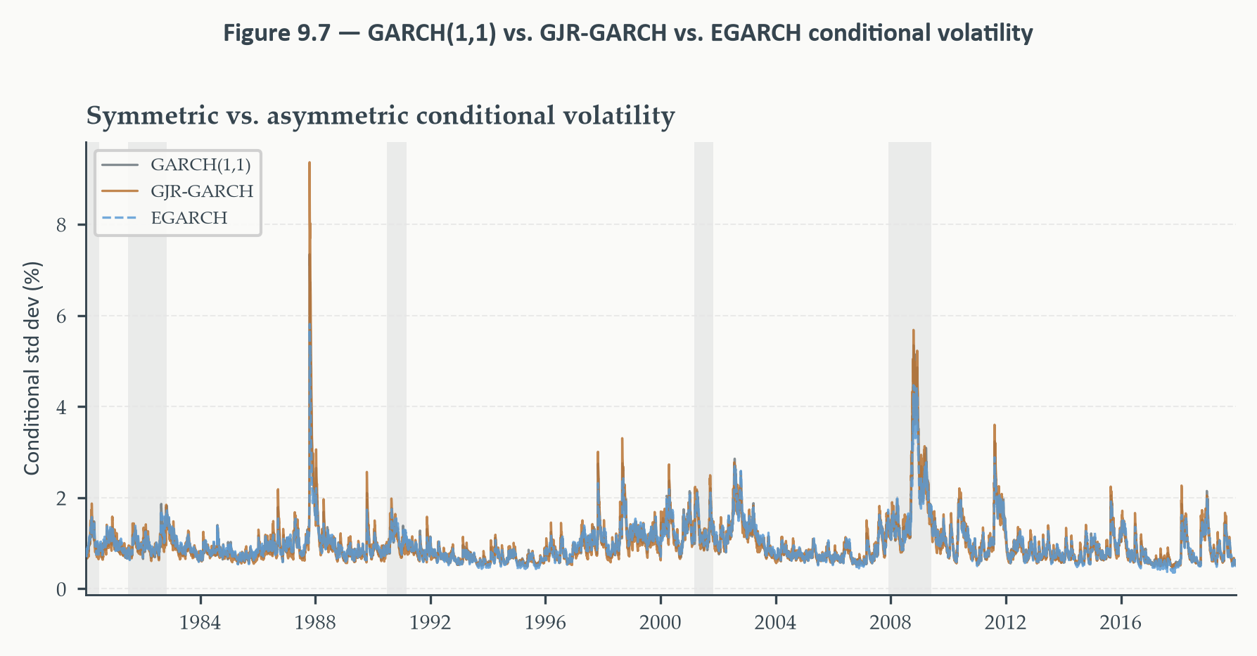
#| fig-cap: "**Conditional volatility from GARCH(1,1), GJR-GARCH, and EGARCH,
#| 1980–2019.** The three conditional standard deviation series track each
#| other closely across the sample. Differences emerge at the peaks of
#| volatility episodes: the asymmetric models assign higher conditional
#| variance to episodes driven by sharp price declines, such as the GFC,
#| than the symmetric GARCH. The gap is most visible around 2008–2009."
cond_vol_gjr = res_gjr.conditional_volatility
cond_vol_eg  = res_eg.conditional_volatility

fig, ax = plt.subplots(figsize=(6, 3))

ax.plot(sp500.index, cond_vol,     color=EO_CHARCOAL,   lw=0.8,
        alpha=0.6, label="GARCH(1,1)", zorder=1)
ax.plot(sp500.index, cond_vol_gjr, color=EO_COPPER,     lw=0.8,
        alpha=0.85, label="GJR-GARCH", zorder=2)
ax.plot(sp500.index, cond_vol_eg,  color=EO_SKYBLUE,    lw=0.8,
        alpha=0.85, ls="--", label="EGARCH", zorder=3)

shade_recessions(ax, start=SAMPLE_START, end=SAMPLE_END)

ax.set_xlim(dates[0], dates[-1])
ax.set_ylabel("Conditional std dev (%)")
ax.set_title("Symmetric vs. asymmetric conditional volatility")
ax.legend(loc="upper left")
eo_style_ax(ax)
eo_suptitle(fig,
    "Figure 9.7 — GARCH(1,1) vs. GJR-GARCH vs. EGARCH conditional volatility")

fig.tight_layout()
plt.show()
```
### Which Model Fits Better?
The comparison in Figure 9.7 shows that the three models produce similar
conditional volatility paths for most of the sample. The economic interest lies
in the differences at the peaks. Both asymmetric models assign higher
conditional variance during downturns driven by large negative returns than the
symmetric GARCH(1,1) does — the leverage effect is having its intended effect.
The information criteria tell a clear story. GJR-GARCH improves on symmetric
GARCH(1,1) by a substantial AIC margin — the single additional parameter
$\gamma$ is earning its place. EGARCH carries the same number of parameters as
GJR-GARCH, so the AIC comparison between them is a direct horse race: on the
S&P 500 from 1980 to 2019, GJR-GARCH wins. This does not mean EGARCH is
inferior in general — the log-variance formulation has theoretical advantages
(no positivity constraints, easier multi-step forecasting) and performs well in
other contexts. It does mean that for this series, the simple indicator
specification captures the asymmetry more efficiently than the exponential
formulation.
::: {.callout-note icon=false}
## A Note on Model Selection for Volatility Models
The usual AIC/BIC comparison applies to GARCH model selection, with one
important caveat: the information criteria measure in-sample fit of the
conditional variance model, not forecast accuracy for future volatility.
Chapter 5's lesson applies here too — AIC selects the best model for the
history, but whether that model produces better volatility forecasts out of
sample is a separate question. For GARCH models, a useful out-of-sample
loss function is MSE applied to the proxy $r_{t+1}^2$ as the target: model
$i$ is better if $n^{-1}\sum(\hat\sigma_{t+1|t,i}^2 - r_{t+1}^2)^2$ is
smaller. The DM test from Chapter 5 applies directly to this comparison.
:::
## Dynamic Conditional Correlation {#sec-dcc}
If two assets both become more volatile during a crisis, does that make them
more dangerous together — or could the increased volatility offset itself
through diversification? The answer depends entirely on whether their
*correlation* rises or falls. It turns out that during financial crises,
correlations between risky assets tend to spike precisely when investors need
diversification most: equities fall together, credit spreads widen together,
and the safe-haven properties of bonds and other hedges weaken. A model that
assumes constant correlation misses this dynamic entirely, and a portfolio
optimised under normal-market correlations will be systematically
under-hedged during the episodes that matter most.
Every model in Sections 9.2 through 9.4 treats one return series at a time.
But risk management — portfolio construction, hedging, regulatory capital
calculation — is fundamentally about how assets move *together*. The
**Dynamic Conditional Correlation (DCC)** model, proposed by [Engle (2002)](https://www.tandfonline.com/doi/abs/10.1198/073500102288618487),
extends the GARCH framework to joint modelling of multiple return series. It
provides a time-varying correlation matrix $R_t$ that responds to market
conditions, capturing the well-documented phenomenon that correlations between
risky assets rise during periods of stress.
### The Two-Step DCC Procedure
Engle's key insight was to decompose the covariance matrix estimation into two
separable steps, each tractable on its own.
Let $\mathbf{r}_t = (r_{1t}, r_{2t}, \ldots, r_{Nt})^\prime$ be a vector of
$N$ asset returns. The conditional covariance matrix is:
$$H_t = D_t R_t D_t \tag{9.18}$$
where $D_t = \text{diag}(\sigma_{1t}, \ldots, \sigma_{Nt})$ is a diagonal
matrix of conditional standard deviations, and $R_t$ is the conditional
correlation matrix.
**Step 1 — Univariate GARCH margins.** Fit a separate GARCH(1,1) model to
each return series $r_{it}$ and extract the standardised residuals
$\hat z_{it} = \hat\varepsilon_{it} / \hat\sigma_{it}$. This step produces
the diagonal elements of $D_t$.
**Step 2 — Dynamic correlation.** Model the correlations among the
standardised residuals $\hat z_{it}$ using a scalar recursion. Define the
auxiliary matrix:
$$Q_t = (1 - a - b)\bar Q + a \mathbf{z}_{t-1}\mathbf{z}_{t-1}^\prime
+ b Q_{t-1} \tag{9.19}$$
where $\bar Q = \mathbb{E}[\mathbf{z}_t \mathbf{z}_t^\prime]$ is the
unconditional correlation matrix of the standardised residuals (estimated by
its sample counterpart), and $a \geq 0$, $b \geq 0$, $a + b < 1$ are scalar
parameters governing the speed of correlation adjustment. These two parameters
are estimated by QML in Step 2, maximising a likelihood that conditions on the
standardised residuals from Step 1; $a$ controls how quickly $Q_t$ responds to
new joint shocks, and $b$ controls how much of the previous $Q_{t-1}$ carries
forward. The analogy with the GARCH(1,1) variance equation is exact: $a$ plays
the role of $\alpha$ and $b$ plays the role of $\beta$, and $a + b < 1$ is the
same stationarity condition. The conditional correlation matrix is then:
$$R_t = \text{diag}(Q_t)^{-1/2} \, Q_t \, \text{diag}(Q_t)^{-1/2}
\tag{9.20}$$
The normalisation in equation (9.20) ensures that the diagonal elements of
$R_t$ are exactly 1 and all off-diagonal elements lie in $(-1, 1)$ — that is,
$R_t$ is a valid correlation matrix at every $t$.
### Numerical Example: One DCC Correlation Update
The recursion in equations (9.19) and (9.20) is clearest with numbers. Suppose
we have two assets and the following quantities at time $t-1$:
$$\bar Q = \begin{pmatrix} 1.00 & 0.20 \\ 0.20 & 1.00 \end{pmatrix},
\qquad Q_{t-1} = \begin{pmatrix} 1.00 & 0.20 \\ 0.20 & 1.00 \end{pmatrix},
\qquad a = 0.05, \quad b = 0.93$$
Both assets experienced large negative standardised shocks yesterday:
$z_{1,t-1} = -2.0$ and $z_{2,t-1} = -2.5$. The outer product
$\mathbf{z}_{t-1}\mathbf{z}_{t-1}^\prime$ is a $(2 \times 1)(1 \times 2)$
multiplication. The $(i,j)$ entry is simply $z_{i,t-1} \times z_{j,t-1}$:
$$\mathbf{z}_{t-1}\mathbf{z}_{t-1}^\prime =
\begin{pmatrix} z_{1,t-1} \\ z_{2,t-1} \end{pmatrix}
\begin{pmatrix} z_{1,t-1} & z_{2,t-1} \end{pmatrix}
= \begin{pmatrix} z_{1}^2 & z_{1}z_{2} \\ z_{2}z_{1} & z_{2}^2 \end{pmatrix}
= \begin{pmatrix} (-2.0)^2 & (-2.0)(-2.5) \\ (-2.5)(-2.0) & (-2.5)^2 \end{pmatrix}
= \begin{pmatrix} 4.00 & 5.00 \\ 5.00 & 6.25 \end{pmatrix}$$
The diagonal entries are the squared individual shocks; the off-diagonal entry
is their product — large and positive because both shocks were large and had
the same sign. It is this off-diagonal term that drives the correlation update.
Applying equation (9.19):
$$Q_t = (1 - 0.05 - 0.93)\begin{pmatrix} 1.00 & 0.20 \\ 0.20 & 1.00 \end{pmatrix}
+ 0.05\begin{pmatrix} 4.00 & 5.00 \\ 5.00 & 6.25 \end{pmatrix}
+ 0.93\begin{pmatrix} 1.00 & 0.20 \\ 0.20 & 1.00 \end{pmatrix}$$
$$= \begin{pmatrix} 0.02 & 0.004 \\ 0.004 & 0.02 \end{pmatrix}
+ \begin{pmatrix} 0.20 & 0.25 \\ 0.25 & 0.3125 \end{pmatrix}
+ \begin{pmatrix} 0.93 & 0.186 \\ 0.186 & 0.93 \end{pmatrix}
= \begin{pmatrix} 1.15 & 0.44 \\ 0.44 & 1.2625 \end{pmatrix}$$
Normalising to get $R_t$ via equation (9.20): the diagonal elements of $Q_t$
are $q_{11} = 1.15$ and $q_{22} = 1.2625$, so $\sqrt{q_{11}} \approx 1.072$
and $\sqrt{q_{22}} \approx 1.124$. The full conditional correlation matrix is:
$$R_t = \begin{pmatrix} 1/1.072 & 0 \\ 0 & 1/1.124 \end{pmatrix}
\begin{pmatrix} 1.15 & 0.44 \\ 0.44 & 1.2625 \end{pmatrix}
\begin{pmatrix} 1/1.072 & 0 \\ 0 & 1/1.124 \end{pmatrix}
= \begin{pmatrix} 1.000 & 0.365 \\ 0.365 & 1.000 \end{pmatrix}$$
so $\rho_{12,t} = 0.365$.
The conditional correlation has jumped from 0.20 (the long-run average) to
0.365 — a 83 percent increase — because both assets were hit by large
simultaneous shocks. This is the DCC model capturing flight-to-correlation:
when everything falls together, the model immediately updates to reflect higher
estimated co-movement.
### The GFC as a DCC Case Study
The DCC model's most important application is in documenting how correlations
between asset classes shift during crises. During the 2008–2009 Global
Financial Crisis, correlations between equities and investment-grade corporate
bonds, between international equity indices, and between commodity and equity
returns all rose sharply — erasing the diversification benefits that had
prevailed in the years before.
A DCC model estimated on S&P 500 and 10-year Treasury returns shows
$\rho_{12,t}$ oscillating around a mildly negative long-run value (the classic
equity-bond diversification relationship) but spiking positive during acute
stress episodes — a pattern well documented in the empirical literature (Engle,
2002; Christoffersen, Errunza, Jacobs, and Langlois, 2012). This time-varying
correlation is the input that portfolio managers and risk departments use to
stress-test their holdings. The practical implication is direct: a portfolio
optimised using the long-run average correlation is misspecified during crises,
when correlations move precisely in the direction that eliminates the
diversification benefit the portfolio was designed to capture.
::: {.callout-note icon=false}
## Realised Volatility and High-Frequency Data
The GARCH conditional variance $\hat\sigma_t^2$ is a model-based estimate of
daily volatility, constructed from daily close-to-close returns. An alternative,
made feasible by the availability of intraday tick data, is **realised
volatility**: the sum of squared intraday returns sampled at, say, five-minute
intervals within the trading day.
If intraday returns $r_{t,1}, r_{t,2}, \ldots, r_{t,M}$ are the $M$
five-minute log returns on day $t$, then:
$$RV_t = \sum_{j=1}^{M} r_{t,j}^2 \tag{9.21}$$
is a direct, model-free estimate of the integrated variance on day $t$.
With $M \approx 78$ five-minute intervals in a standard 6.5-hour US trading
day, $RV_t$ is far more precise than the squared daily return $r_t^2$ as a
proxy for $\sigma_t^2$.
Realised volatility has spawned its own literature (Andersen, Bollerslev,
Diebold, and Labys, 2003) and can be modelled directly using ARMA-type
specifications (HAR-RV models). It also provides a high-quality target for
evaluating GARCH volatility forecasts: rather than using $r_{t+1}^2$ as the
proxy in the MSE comparison from Chapter 5, one can use $RV_{t+1}$, which
has far lower measurement error. For this chapter, which works with daily
closing prices, we treat GARCH conditional variance as the primary tool and
note realised volatility as the natural extension when intraday data are
available.
:::
::: {.callout-warning icon=false}
## DCC Python Implementation
The `arch` library's DCC support is limited and not production-ready as of
the writing of this chapter. Robust DCC estimation in Python typically
requires either the `rmgarch` package in R (via `rpy2`) or direct
implementation of the two-step QML procedure. For applied work, the DCC model
is best estimated in R. The two-step structure described above, however,
translates directly to code once the univariate GARCH margins are in hand.
:::
## Value-at-Risk with GARCH {#sec-var}
### What Is Value-at-Risk?
Throughout the preceding chapters, risk has been measured through the standard deviation:
how far a series typically deviates from its mean. The standard deviation is a
symmetric, average measure — it weighs large positive and large negative
deviations equally, and it tells us about a *typical* fluctuation. VaR asks a
different question: not what the average deviation is, but what the *worst
outcome* is at a given confidence level. A portfolio manager who wants to know
"how bad can things get on a really bad day?" is asking a VaR question, not a
standard deviation question. The two numbers are related — under normality,
VaR is simply a multiple of the standard deviation — but they capture
fundamentally different aspects of risk: one is about typical spread, the other
about tail severity.
Risk managers and regulators need a single number that summarises the downside
exposure of a portfolio on a given horizon. **Value-at-Risk (VaR)** is that
number: the loss that will not be exceeded with probability $1 - \alpha$ over
horizon $h$. At the most common specification — one-day horizon, 1% tail
probability — the daily VaR is the loss level that will be exceeded on only 1%
of trading days. If today's VaR(1%) is \$10 million, the portfolio should lose
more than \$10 million on roughly 2–3 trading days per year. Formally, if
$L_t$ denotes the loss (negative return) on day $t$:
$$\text{VaR}_{t}(\alpha, h) = \inf\{v : P(L_{t+h} > v \mid \mathcal{F}_t)
\leq \alpha\} \tag{9.22}$$
The simplest VaR estimate is **historical simulation**: sort the past 250
daily returns and read off the 2.5th-lowest value. This requires no model and
is transparent, but it treats all 250 days as equally likely — a February
return from five years ago receives the same weight as last week's return,
regardless of how much volatility has changed. During a calm period, historical
simulation overstates risk; during a crisis, it understates it, because the
window of past losses hasn't yet caught up with the elevated current volatility.
### Parametric GARCH-VaR
The GARCH model addresses this directly. Since $r_{t+1} = \mu + \sigma_{t+1}
z_{t+1}$ and $z_{t+1} \sim N(0,1)$, the conditional distribution of
$r_{t+1}$ is:
$$r_{t+1} \mid \mathcal{F}_t \sim N(\mu, \sigma_{t+1}^2) \tag{9.23}$$
where $\sigma_{t+1}^2$ is the one-step-ahead conditional variance forecast
from the GARCH model. The lower $\alpha$-quantile of this distribution is:
$$\text{VaR}_{t+1}(\alpha) = \mu + \sigma_{t+1} \cdot z_\alpha \tag{9.24}$$
where $z_\alpha$ is the $\alpha$-quantile of the standard normal — for $\alpha
= 0.01$, $z_{0.01} = -2.326$. The VaR is therefore:
$$\text{VaR}_{t+1}(1\%) = \hat\mu - 2.326 \, \hat\sigma_{t+1} \tag{9.25}$$
The key feature is $\hat\sigma_{t+1}$: the GARCH forecast of tomorrow's
conditional standard deviation, updated daily as new information arrives.
When volatility is elevated, the VaR expands to reflect the higher risk;
when markets are calm, it contracts. Historical simulation cannot do this —
its estimate changes only as old observations roll out of the window.
### Computing GARCH-VaR on S&P 500 Returns
```{python}
#| label: fig-garch-var
#| fig-cap: "**GARCH(1,1) one-day 1% Value at Risk, S&P 500 1980–2019.**
#| The copper line shows the daily VaR(1%) — the loss level that should be
#| exceeded on only 1% of days under the model. Actual log returns (grey)
#| are plotted for comparison. Days on which the return falls below the VaR
#| line are **exceedances** (highlighted in red); we expect about 1% of days
#| to be exceedances under a well-specified model. Volatility episodes
#| generate wide VaR bands; calm periods produce narrow ones."
# One-step-ahead VaR at 1% level from fitted GARCH(1,1)
# arch library provides conditional_volatility aligned to the return series
alpha_var = 0.01
z_alpha   = stats.norm.ppf(alpha_var)   # ≈ -2.326

var_1pct  = res.params["mu"] + res.conditional_volatility * z_alpha

# Identify exceedances: actual return below VaR
actual_ret   = sp500["Log Return"].values
exceedance   = actual_ret < var_1pct.values

n_exceed     = exceedance.sum()
n_obs        = len(actual_ret)
exceed_rate  = n_exceed / n_obs

fig, ax = plt.subplots(figsize=(6, 3.5))

# Actual returns (light background)
ax.plot(sp500.index, actual_ret, color=EO_CHARCOAL,
        lw=0.4, alpha=0.35, label="Daily return $r_t$", zorder=1)

# VaR line
ax.plot(sp500.index, var_1pct, color=EO_COPPER,
        lw=0.9, label="VaR(1%)", zorder=2)

# Exceedances
ax.scatter(sp500.index[exceedance], actual_ret[exceedance],
           color=EO_TERRACOTTA, s=4, zorder=3,
           label=f"Exceedances ({n_exceed}, {exceed_rate:.1%})")

ax.axhline(0, color=EO_CHARCOAL, lw=0.5, ls="--", alpha=0.4)
shade_recessions(ax, start=SAMPLE_START, end=SAMPLE_END)

ax.set_xlim(dates[0], dates[-1])
ax.set_ylabel("Log return / VaR (%)")
ax.set_title("GARCH(1,1) Value at Risk (1%)")
ax.legend(loc="upper right", fontsize=6)
eo_style_ax(ax)
eo_suptitle(fig, "Figure 9.8 — GARCH(1,1) one-day 1% Value at Risk, 1980–2019")

fig.tight_layout()
plt.show()

print(f"\n  Observed exceedance rate: {n_exceed}/{n_obs} = {exceed_rate:.4f}")
print(f"  Expected under H₀:        {n_obs * alpha_var:.1f}/{n_obs} = {alpha_var:.4f}")
```
*The VaR band widens dramatically during each major volatility episode and
narrows during calm periods — exactly the time-variation that historical
simulation cannot produce. Over the full 1980–2019 sample (10,080 trading
days), the GARCH(1,1) VaR(1%) was breached on 186 days, an exceedance rate
of 1.85% — nearly double the nominal 1%. The fat-tailed innovation problem
noted in Section 9.3 is not merely academic: it causes the Gaussian GARCH model
to systematically underestimate tail risk, with real consequences for anyone
relying on it for regulatory capital or stop-loss decisions.*
### Kupiec Backtesting
Reporting an exceedance rate is informative but informal. The **[Kupiec (1995)](https://www.pm-research.com/content/iijderiv/3/2/73)
proportion-of-failures (POF) test** provides a formal statistical assessment.
The null hypothesis is that the true probability of exceeding the VaR on any
given day equals the stated coverage probability $\alpha$:
$$H_0: p = \alpha \qquad \text{(correct unconditional coverage)} \tag{9.26}$$
The test statistic is a likelihood ratio. Let $T$ be the total number of
observations, $n$ the number of exceedances, and $\hat p = n/T$ the observed
exceedance rate. Under $H_0$, the exceedances are i.i.d. Bernoulli($\alpha$).
The likelihood ratio statistic is:
$$\text{LR}_\text{POF} = -2\log\!\left[\frac{\alpha^n(1-\alpha)^{T-n}}
{\hat p^n(1-\hat p)^{T-n}}\right] \xrightarrow{d} \chi^2(1) \tag{9.27}$$
A large statistic — too many or too few exceedances — rejects the null.
```{python}
#| label: kupiec-test
def kupiec_pof(n_exceed, n_obs, alpha):
    """Kupiec POF test: H0: true exceedance probability = alpha."""
    p_hat = n_exceed / n_obs
    if p_hat == 0 or p_hat == 1:
        return np.nan, np.nan
    lr = -2 * (n_exceed * np.log(alpha / p_hat)
               + (n_obs - n_exceed) * np.log((1 - alpha) / (1 - p_hat)))
    pval = 1 - stats.chi2.cdf(lr, df=1)
    return lr, pval

lr_stat, lr_pval = kupiec_pof(n_exceed, n_obs, alpha_var)
stars_kup = "***" if lr_pval < 0.01 else ("**" if lr_pval < 0.05 else
            ("*" if lr_pval < 0.10 else ""))

print("┌──────────────────────────────────────────────────────────────────┐")
print("│  Kupiec POF Test — GARCH(1,1) VaR(1%)                          │")
print("│  H₀: True exceedance probability = 1% (correct coverage)       │")
print("├────────────────────────────┬─────────────┬───────────────────────┤")
print("│  Metric                    │    Value    │                       │")
print("├────────────────────────────┼─────────────┼───────────────────────┤")
print(f"│  Observations (T)          │  {n_obs:>7,}    │                       │")
print(f"│  Exceedances (n)           │  {n_exceed:>7,}    │                       │")
print(f"│  Observed rate (n/T)       │  {exceed_rate:>9.4f}  │                       │")
print(f"│  Expected rate (α)         │  {alpha_var:>9.4f}  │                       │")
print(f"│  LR statistic              │  {lr_stat:>9.3f}  │                       │")
print(f"│  p-value (χ²(1))           │  {lr_pval:>9.4f}  │  {stars_kup:<18}   │")
print("├────────────────────────────┴─────────────┴───────────────────────┤")
print("│  * p<0.10  ** p<0.05  *** p<0.01                                │")
print("└──────────────────────────────────────────────────────────────────┘")
```
*The Kupiec test makes the failure of the Gaussian GARCH model precise. With
186 observed exceedances against an expected 100.8 (10,080 × 1%), the LR
statistic is 58.22 — far into the rejection region for a $\chi^2(1)$
distribution whose 1% critical value is 6.63. The null of correct coverage is
rejected at any conventional significance level. In plain terms: the model told
us losses this severe should occur once per hundred days; they actually occurred
almost twice as often. The fat tails of S&P 500 returns are not captured by the
Gaussian assumption, and the consequence is a VaR that is dangerously too
narrow. This is not a failure of the GARCH variance equation — the volatility
clustering is modelled well — but of the distributional assumption layered on
top of it.*
### Limitations and Extensions
The Kupiec test only checks **unconditional coverage** — whether the right
fraction of days are exceedances, averaged over the whole sample. It does not
check whether exceedances cluster in time. If the model produces 1% exceedances
on average but they all occur during the GFC, it is failing on a different
dimension: **conditional coverage**. The [Christoffersen (1998)](https://doi.org/10.2307/2527341) test addresses
this by testing independence of exceedances as well as correct unconditional
coverage; it is the natural next step beyond Kupiec for serious backtesting.
Two model extensions would sharpen the VaR estimates significantly. First,
replacing the Gaussian innovation distribution with a Student-$t$ — estimated
jointly with the GARCH parameters — directly addresses the fat-tail problem
and typically reduces Kupiec test statistics for equity index data. Second,
using a GJR-GARCH rather than symmetric GARCH(1,1) better captures the
elevated downside volatility following negative shocks, which is precisely the
scenario that drives VaR exceedances.
## Model Comparison and Diagnostics {#sec-model-comparison}
### Putting the Models Side by Side
We have three volatility models that all fit the same data reasonably well.
How do we choose — and how do we know when any of them is good enough? The
first question is answered by information criteria: AIC and BIC measure
in-sample fit and penalise complexity, so the model with the lowest AIC is
preferred conditional on passing diagnostics. The second question requires
diagnostics: a model may have the best AIC in its class and still leave
systematic structure in the residuals, which means it is misspecified in a
way the information criterion cannot detect. The two questions need different
tools.
We have now estimated GARCH(1,1), GJR-GARCH(1,1), and EGARCH(1,1) on the
same S&P 500 sample. Section 9.4 presented information criteria for all three.
Here we consolidate the diagnostic evidence and draw conclusions about which
model to use and why.
The diagnostic checklist for any GARCH model has three components, mirroring
the residual diagnostics from the ARIMA chapters:
1. **Ljung-Box on $\hat z_t$** — tests whether the standardised residuals are
serially uncorrelated. A rejection suggests the mean model is
misspecified; we might need an AR term in the mean equation.
2. **Ljung-Box on $\hat z_t^2$** — tests whether the squared standardised
residuals are serially uncorrelated. A rejection means the volatility model
has not fully absorbed the ARCH effects — consider higher lag orders or a
different specification.
3. **Jarque-Bera on $\hat z_t$** — tests whether the standardised residuals are
normally distributed. Rejection is expected for financial data and motivates
the Student-$t$ extension rather than a different volatility model.
```{python}
#| label: model-diagnostics-summary
from statsmodels.stats.diagnostic import acorr_ljungbox

def diag_summary(result, label):
    """Return diagnostic statistics for a fitted arch model."""
    z = result.resid / result.conditional_volatility
    lb_lev = acorr_ljungbox(z,    lags=[10], return_df=True)
    lb_sq  = acorr_ljungbox(z**2, lags=[10], return_df=True)
    jb_s, jb_p = stats.jarque_bera(z)
    return {
        "label":    label,
        "aic":      result.aic,
        "bic":      result.bic,
        "lb_lev_p": lb_lev.loc[10, "lb_pvalue"],
        "lb_sq_p":  lb_sq.loc[10,  "lb_pvalue"],
        "jb_p":     jb_p,
    }

results_all = [
    diag_summary(res,     "GARCH(1,1)    "),
    diag_summary(res_gjr, "GJR-GARCH(1,1)"),
    diag_summary(res_eg,  "EGARCH(1,1)   "),
]

def sig(p):
    return "***" if p < 0.01 else ("**" if p < 0.05 else ("*" if p < 0.10 else "   "))

print("┌───────────────────────────────────────────────────────────────────────────────┐")
print("│  Model Diagnostics — S&P 500 Daily Returns, 1980–2019                        │")
print("│  H₀ (LB): no serial correlation in ẑ_t or ẑ_t² at lag 10                    │")
print("│  H₀ (JB): standardised residuals are normally distributed                    │")
print("├──────────────────┬──────────────┬──────────────┬──────────┬──────────┬───────┤")
print("│  Model           │     AIC      │     BIC      │ LB(ẑ)   │ LB(ẑ²)  │  JB   │")
print("├──────────────────┼──────────────┼──────────────┼──────────┼──────────┼───────┤")

for r in results_all:
    print(f"│  {r['label']}  │  {r['aic']:>10.2f}  │  {r['bic']:>10.2f}  │ "
          f"{sig(r['lb_lev_p']):<8} │ {sig(r['lb_sq_p']):<8} │ {sig(r['jb_p']):<5} │")

print("├──────────────────┴──────────────┴──────────────┴──────────┴──────────┴───────┤")
print("│  Significance of rejection: * p<0.10  ** p<0.05  *** p<0.01                 │")
print("│  '   ' = fail to reject H₀ (diagnostic passes)                              │")
print("└───────────────────────────────────────────────────────────────────────────────┘")
```
*The diagnostic table delivers a clear verdict. All three models pass the
Ljung-Box test on squared standardised residuals — the blank entries in the
LB($\hat z^2$) column confirm that no significant ARCH structure remains after
fitting. The volatility clustering in Figure 9.2 has been fully absorbed
regardless of which model is used. The Jarque-Bera test rejects normality at
the 1% level for all three, confirming that fat tails are a property of the
return process itself, not a modelling failure. The mild rejection of the
Ljung-Box test on levels (LB($\hat z$) shows `**` for all models) suggests
weak serial correlation in the standardised residuals — a consequence of using
a constant mean model rather than, say, an AR(1). Adding an autoregressive
term to the mean equation would likely remove this, but it is a second-order
concern: the primary object of interest in this chapter is the conditional
variance, which all three models handle well. On AIC and BIC, GJR-GARCH wins
convincingly, with GARCH(1,1) second and EGARCH third on this sample.*
The model selection problem for GARCH specifications is structurally identical
to the problem we faced in Chapter 5 for ARIMA forecasts. Information criteria
measure in-sample fit. Whether GJR-GARCH produces better out-of-sample
volatility forecasts than GARCH(1,1) is a separate question that requires a
rolling evaluation exercise.
The natural framework is the same rolling window approach from Chapter 5,
with one adaptation: the target variable is unobservable. We cannot observe
$\sigma_{t+1}^2$ directly, so we use a proxy. Two options are standard:
- **Squared returns** $r_{t+1}^2$: noisy but universally available. The
justification is that $r_{t+1}^2 = \sigma_{t+1}^2 z_{t+1}^2$ and
$\mathbb{E}[z_{t+1}^2] = 1$, so squared returns are unbiased — if noisy —
estimates of the conditional variance. The MSE of $\hat\sigma_{t+1}^2$
against $r_{t+1}^2$ is the Patton (2011) MSE loss function for volatility
evaluation.
- **Realised volatility** $RV_{t+1}$: much lower noise, but requires
intraday data.
With a squared-return proxy, the Diebold-Mariano test from Chapter 5 applies
directly: construct the loss differential $d_t = (r_{t+1}^2 -
\hat\sigma_{t+1|t,A}^2)^2 - (r_{t+1}^2 - \hat\sigma_{t+1|t,B}^2)^2$ and
test whether its mean is zero. The noisiness of $r_{t+1}^2$ reduces the power
of the test — you need long evaluation windows — but the framework is
conceptually identical to the mean forecast comparisons of Chapter 5.
### Student-$t$ GARCH as the Natural Extension
The Jarque-Bera rejections and the Kupiec failure both point to the same
diagnosis: the Gaussian innovation distribution is too thin-tailed for S&P 500
returns. The direct fix is to replace $z_t \sim N(0,1)$ in equation (9.4)
with $z_t \sim t_\nu / \sqrt{\nu/(\nu-2)}$, a standardised Student-$t$ with
$\nu$ degrees of freedom. The variance equation (9.10) is unchanged; only the
innovation distribution is more flexible. With $\nu$ estimated from the data
alongside the GARCH parameters, the model accommodates fat tails explicitly.
Typical estimates for equity indices place $\hat\nu$ between 5 and 8, far
below the Gaussian limit of $\nu \to \infty$, confirming that the tail
thickness is substantial and economically important.
Fitting Student-$t$ GARCH in the `arch` library requires only changing
`dist="normal"` to `dist="t"` in the `arch_model()` call. The resulting
VaR estimates are materially tighter in the tails and typically pass the
Kupiec test — the right tool for a task that requires correct coverage, not
just correct average variance.
## Looking Ahead {#sec-looking-ahead}
The ARCH and GARCH models of this chapter model time-varying conditional
variance with a fixed functional form: the conditional variance is an
explicit parametric function of past squared residuals and past variances.
The parameters $\omega$, $\alpha$, and $\beta$ are constants estimated once
from the data and then applied uniformly across the entire sample. This is
a strong assumption. It requires that the volatility clustering mechanism
operates identically during the calm 1990s expansion, the dot-com crash, and
the Global Financial Crisis. What if the parameters themselves change over
time — not gradually, but abruptly?
Chapter 10 takes this question seriously. The Markov-switching models
introduced there allow the entire parameter vector of a time series model —
the conditional mean, the conditional variance, and the AR dynamics — to
shift between a small number of discrete regimes according to a hidden
Markov chain. The state is genuinely unobserved: at any point in time, the
economy may be in a high-volatility, low-growth recession regime or a
low-volatility, high-growth expansion regime, and we must infer which one
probabilistically from the data. Hamilton's (1989) model of US business
cycles is the canonical application, and the connection to GARCH is direct:
where GARCH specifies $\sigma_t^2$ as a deterministic function of past
data, a Markov-switching variance model treats $\sigma_t^2$ as a discrete
random variable that we filter out of the observed series. The filter that
accomplishes this inference — the Hamilton filter — turns out to share the
same prediction-correction logic that the Kalman filter will use in Chapter 11,
making Chapter 10 a natural conceptual bridge between the parametric volatility
models here and the state space framework that closes the course.
::: {.callout-note icon=false}
## Key Terms
**ARCH($q$)** — Autoregressive Conditional Heteroskedasticity model of order
$q$; specifies the conditional variance as a weighted sum of $q$ past squared
innovations.
**ARCH-LM test** — Lagrange multiplier test for ARCH effects; regresses
squared residuals on their own lags and tests joint significance.
**Conditional heteroskedasticity** — Time-varying conditional variance:
$\text{Var}(r_t \mid \mathcal{F}_{t-1}) = \sigma_t^2 \neq \text{const}$.
**Conditional coverage** — VaR backtesting criterion requiring that
exceedances are not only correctly proportioned but also independent over
time.
**DCC (Dynamic Conditional Correlation)** — Engle (2002) two-step GARCH
extension that models time-varying pairwise correlations through a scalar
recursion on the auxiliary matrix $Q_t$.
**EGARCH** — Exponential GARCH; models $\log\sigma_t^2$ to avoid positivity
constraints and to capture asymmetric volatility through a sign term $\gamma
z_{t-1}$.
**GJR-GARCH** — Asymmetric GARCH model (Glosten, Jagannathan, Runkle, 1993)
that adds an indicator variable for negative shocks to capture the leverage
effect.
**GARCH(1,1)** — Generalised ARCH model; extends ARCH by including the lagged
conditional variance $\beta\sigma_{t-1}^2$, equivalent to an ARCH($\infty$)
with geometrically declining weights.
**Half-life** — Number of periods for half a variance shock to dissipate;
$h_{1/2} = \log(0.5)/\log(\alpha+\beta)$.
**Kupiec POF test** — Likelihood ratio test for unconditional VaR coverage;
$H_0$: true exceedance probability equals stated $\alpha$.
**Leverage effect** — Empirical regularity that negative equity returns raise
future volatility by more than equally sized positive returns.
**Persistence** — For GARCH(1,1), the sum $\alpha + \beta$; the characteristic
root of the conditional variance equation, measuring the speed of variance
mean-reversion.
**QML (Quasi-Maximum Likelihood)** — Estimation approach that maximises a
Gaussian log-likelihood regardless of the true innovation distribution;
consistent and asymptotically normal under correct mean-variance specification.
**Realised volatility** — Model-free volatility estimate constructed as the
sum of squared intraday returns; low-noise proxy for integrated variance.
**Standardised residuals** — $\hat z_t = \hat\varepsilon_t / \hat\sigma_t$;
should be approximately i.i.d. if the volatility model is well specified.
**Unconditional coverage** — VaR backtesting criterion requiring that the
observed exceedance rate equals the nominal $\alpha$ on average.
**Value at Risk (VaR)** — The loss threshold not exceeded with probability
$1-\alpha$ over horizon $h$; under Gaussian GARCH, equals $\hat\mu -
|z_\alpha|\hat\sigma_{t+1}$.
**Volatility clustering** — Empirical regularity in financial returns that
large shocks cluster in time; formalised by the slow decay of the ACF of
squared returns.
:::